Usage

• 1: Indexing
• 2: Multi-Vector Retrieval
• 3: Graph Index
• 4: Quantization Types
• 5: Similarity Filter
• 6: PostgreSQL Tuning
• 7: Monitoring
• 8: Fallback Parameters
• 9: Measure Recall
• 10: Prewarm
• 11: Prefilter
• 12: Prefetch
• 13: Rerank in Table
• 14: Partitioning Tuning
• 15: External Build

1 - Indexing

VectorChord’s index type vchordrq divides vectors into lists and searches only a subset of lists closest to the query vector. It provides fast build time and low memory consumption, while delivering significantly better performance than both hnsw and ivfflat.

Let’s start by creating a table named items with an embedding column of type vector(n), and then populate it with sample data.

CREATE TABLE items (id bigserial PRIMARY KEY, embedding vector(3));
INSERT INTO items (embedding) SELECT ARRAY[random(), random(), random()]::real[] FROM generate_series(1, 1000);

To create a vchordrq index, you can use the following SQL.

CREATE INDEX ON items USING vchordrq (embedding vector_l2_ops);

After the index is built, you can perform a vector search using it to retrieve the $10$ nearest neighbors to a vector.

SELECT * FROM items ORDER BY embedding <-> '[3,1,2]' LIMIT 10;

You can also add filters to vector search queries as needed.

SELECT * FROM items WHERE id % 7 <> 0 ORDER BY embedding <-> '[3,1,2]' LIMIT 10;

Tuning

When there are less than $100,000$ rows in the table, you usually don’t need to set the index options.

CREATE INDEX ON items USING vchordrq (embedding vector_l2_ops);

SELECT * FROM items ORDER BY embedding <-> '[3,1,2]' LIMIT 10;

However, as the number of rows grows, partitioning becomes necessary and can be configured using index options. options are specified using a TOML: Tom’s Obvious Minimal Language string. You can refer to #Index Options for more information.

CREATE INDEX ON items USING vchordrq (embedding vector_l2_ops) WITH (options = $$
[build.internal]
lists = [1000]
$$);

SET vchordrq.probes TO '10';
SELECT * FROM items ORDER BY embedding <-> '[3,1,2]' LIMIT 10;

The parameter lists should be tuned based on the number of rows. The following table provides guidelines for choosing an appropriate value. When querying, choose vchordrq.probes accordingly.

The process of building an index involves two steps: partitioning the vector space first, and then inserting rows into the index. The first step, partitioning the vector space, can be sped up using multiple threads.

CREATE INDEX ON items USING vchordrq (embedding vector_l2_ops) WITH (options = $$
[build.internal]
lists = [1000]
build_threads = 8
$$);

SET vchordrq.probes TO '10';
SELECT * FROM items ORDER BY embedding <-> '[3,1,2]' LIMIT 10;

The second step, inserting rows, can be parallelized using multiple processes. Refer to PostgreSQL Tuning.

For most datasets using cosine similarity, enabling residual_quantization and build.internal.spherical_centroids improves both QPS and recall.

CREATE INDEX ON items USING vchordrq (embedding vector_cosine_ops) WITH (options = $$
residual_quantization = true
[build.internal]
lists = [1000]
spherical_centroids = true
build_threads = 8
$$);

SET vchordrq.probes TO '10';
SELECT * FROM items ORDER BY embedding <=> '[3,1,2]' LIMIT 10;

To improve the build speed, you may opt to use more shared memory to accelerate the process by setting build.pin to 2.

CREATE INDEX ON items USING vchordrq (embedding vector_l2_ops) WITH (options = $$
residual_quantization = true
build.pin = 2
[build.internal]
lists = [1000]
spherical_centroids = true
build_threads = 8
$$);

For large tables, time and memory overhead are dominated by the partitioning phase. See Partitioning Tuning for further tuning.

You can also refer to External Build to offload the partitioning phase to other machines.

Reference

Operator Classes (vchordrq)

The following table lists all available operator classes supported by vchordrq.

<->, <#> and <=> are operators defined by pgvector.

<<->>, <<#>>, <<=>> are operators defined by VectorChord. For more information about <<->>, <<#>>, <<=>>, refer to Similarity Filter.

@# is an operator defined by VectorChord. For more information about @#, refer to Multi-Vector Retrieval.

rabitq8, rabitq4 are types defined by VectorChord. For more information about rabitq8, rabitq4, refer to Quantization Types.

The operator classes for MaxSim are available since version 0.3.0. The operator classes for rabitq8 and rabitq4 are available since version 1.1.0.

Indexing Options (vchordrq)

residual_quantization

• Description: This option determines whether residual quantization is used. If you are not familiar with residual quantization, you can read this blog for more information. In short, residual quantization is a technique that improves the accuracy of vector search by quantizing the residuals of the vectors.
• Type: boolean
• Default: false
• Example:
  • residual_quantization = false means that residual quantization is not used.
  • residual_quantization = true means that residual quantization is used.
• Note: This option is not supported for rabitq8 and rabitq4.

degree_of_parallelism

• Description: This option is a hint that specifies the degree of parallelism. In most cases, you do not need to change it. If you are using a CPU with more than 32 threads and wish to utilize more threads for PostgreSQL, you may set it to the number of threads for better performance.
• Type: integer
• Default: 32
• Domain: [1, 256]
• Example:
  • degree_of_parallelism = 32 hints to the index that 32 or less processes may access on the index concurrently.
  • degree_of_parallelism = 64 hints to the index that 64 or less processes may access on the index concurrently.

build.pin

• Description: This option determines whether shared memory is used for indexing. For large tables, you can choose to enable this option to speed up the build process.
• Type: union of integer and boolean
• Default:
  • -1 since v1.0.0
  • false until v0.5.3
• Domain:
  • {-1, 0, 1, 2, false, true} since v1.0.0
  • {false, true} until v0.5.3
• Example:
  • build.pin = 2 means the hot portion of the index is cached in memory.
  • build.pin = 1 means a subset of the hot portion of the index is cached in memory, consuming less memory.
  • build.pin = 0 means that this feature is enabled but nothing is actually cached. This option is for debugging purposes only.
  • build.pin = -1 means that this feature is disabled.
  • build.pin = false is the legacy form of build.pin = -1.
  • build.pin = true is the legacy form of build.pin = 1.

Default Build Options

This is the default value of index building. The index will not be partitioned. In terms of semantics, build.default = {} is similar to build.internal.lists = [].

Internal Build Options (vchordrq)

build.internal.lists

• Description: This option determines the hierarchical structure of the vector space partitioning.
• Type: list of integers
• Default:
  • [] since v0.3.0
  • [1000] until v0.2.2: implicit behavior is not ideal
• Example:
  • build.internal.lists = [] means that the vector space is not partitioned.
  • build.internal.lists = [4096] means the vector space is divided into $4096$ cells.
  • build.internal.lists = [4096, 262144] means the vector space is divided into $4096$ cells, and those cells are further divided into $262144$ smaller cells.
• Note: The index partitions the vector space into multiple Voronoi cells based on centroids, iteratively creating a hierarchical space partition tree. Each leaf node in this tree represents a region with an associated list storing vectors in that region. During insertion, vectors are placed in lists corresponding to their appropriate leaf nodes. For queries, the index optimizes search by excluding lists whose leaf nodes are distant from the query vector, effectively pruning the search space. If the length of lists is $1$, the lists option should be no less than $4\sqrt{N}$, where $N$ is the number of vectors in the table.

build.internal.spherical_centroids

• Description: This option determines whether to perform spherical K-means – the centroids are L2 normalized after each iteration, you can refer to option spherical in here.
• Type: boolean
• Default: false
• Example:
  • build.internal.spherical_centroids = false means that spherical k-means is not performed.
  • build.internal.spherical_centroids = true means that spherical k-means is performed.
• Note: Set this to true if your model generates embeddings that use cosine similarity as the metric.

build.internal.sampling_factor

• Description: This option determines the number of vectors the K-means algorithm samples per cluster. The higher this value, the slower the build, the greater the memory consumption in building, and the better search performance.
• Type: integer
• Domain: [0, 1024]
• Default: 256
• Example:
  • build.internal.sampling_factor = 256 means that the K-means algorithm samples $256 C$ vectors, where $C$ is the maximum value in build.internal.lists.
  • build.internal.sampling_factor = 32 means that the K-means algorithm samples $32 C$ vectors, where $C$ is the maximum value in build.internal.lists. This reduces K-means’ time and memory usage to approximately $\frac{1}{8}$ of what it would be with the default value of 256.

build.internal.kmeans_iterations

• Description: This option determines the number of iterations for K-means algorithm. The higher this value, the slower the build.
• Type: integer
• Domain: [0, 1024]
• Default: 10
• Example:
  • build.internal.kmeans_iterations = 10 means that the K-means algorithm performs $10$ iterations.
  • build.internal.kmeans_iterations = 100 means that the K-means algorithm performs $100$ iterations.

build.internal.build_threads

• Description: This option determines the number of threads used by K-means algorithm. The higher this value, the faster the build, and greater load on the server in building.
• Type: integer
• Domain: [1, 255]
• Default: 1
• Example:
  • build.internal.build_threads = 1 means that the K-means algorithm uses $1$ thread.
  • build.internal.build_threads = 4 means that the K-means algorithm uses $4$ threads.

build.internal.kmeans_algorithm

• Description: This option determines the K-means algorithm to be used.
• Type: object
• Example:
  • build.internal.kmeans_algorithm.lloyd = {}. This uses Lloyd’s algorithm. This is the default value.
  • build.internal.kmeans_algorithm.hierarchical = {}. This uses hierarchical clustering. Compared to Lloyd’s algorithm, this approach is much faster, but it may cause a loss of accuracy.

build.internal.kmeans_dimension

• Description: This option determines the dimension to use for K-means input and output. This feature employs dimensionality reduction and expansion via resampling, effectively reducing K-means’ time and memory consumption, but it may cause a loss of accuracy.
• Type: union of integer and null
• Default: null
• Example:
  • If this option is not set, this feature is disabled.
  • build.internal.kmeans_dimension = 100 means that K-means will process vectors with $100$ dimensions. For original vectors of $900$ dimensions, this reduces K-means’ time and memory usage to approximately $\frac{1}{9}$ of what it would be without this feature.

Search Parameters (vchordrq)

vchordrq.enable_scan

• Description: Enables or disables the query planner’s use of vchordrq index scan. It’s for testing purposes.
• Type: boolean
• Default: on
• Example:
  • vchordrq.enable_scan = off disables the query planner’s use of vchordrq index scan.
  • vchordrq.enable_scan = on enables the query planner’s use of vchordrq index scan.

vchordrq.probes

• Description: This GUC parameter vchordrq.probes controls how the vector space assists in query pruning. The more probes, the more accurate the search, but also the slower it is.
• Type: list of integers
• Default:
  • since v0.3.0
  • 10 until v0.2.2: the default value was 10 before `lists` defaulted to empty
  • This parameter supports fallback.
• Example:
  • SET vchordrq.probes = 1 means that only one probe is used.
  • SET vchordrq.probes = 10 means that ten probes are used.
• Note: The default value is an empty list. The length of this option must match the length of lists.
  • If lists = [], then probes must be .
  • If lists = [11, 22], then probes can be 2,4 or 4,8. It must not be incorrectly shaped, for example, , 3, 7,8,9, 5,5,5,5.

vchordrq.epsilon

• Description: Even after pruning, the number of retrieved vectors remains substantial. The index employs the RaBitQ algorithm to quantize vectors into bit vectors, which require just $\frac{1}{32}$ the memory of single-precision floating-point vectors. Most computations are integer-based, leading to faster processing. Unlike conventional quantization algorithms, RaBitQ estimates not only distances but also their lower bounds. The index computes the lower bound for each vector and dynamically adjusts the number of vectors needing recalculated distances, based on the query count, thus balancing performance and accuracy. The GUC parameter vchordrq.epsilon controls the conservativeness of the lower bounds of distances. The higher the value, the higher the accuracy, but the worse the performance. The default value tends to favor higher accuracy than needed for most use cases, so you can try lowering this parameter to achieve better performance.
• Type: real
• Default:
  • 1.9
  • This parameter supports fallback.
• Domain: [0.0, 4.0]
• Example:
  • SET vchordrq.epsilon = 0.1 indicates you are using a very optimistic lower bound estimation. You set it this way because your dataset is not sensitive to the lower bound estimation, for the precision you need.
  • SET vchordrq.epsilon = 4.0 indicates you are using a very pessimistic lower bound estimation. You set it this way because your dataset is not very sensitive to the lower bound estimation, for the precision you need.

vchordrq.prewarm_dim

• Description: The vchordrq.prewarm_dim GUC parameter is used to precompute the RaBitQ projection matrix for the specified dimensions. This can help to reduce the latency of the first query after the PostgreSQL cluster is started.
• Type: list of integers
• Default: 64,128,256,384,512,768,1024,1536
• Example:
  • ALTER SYSTEM SET vchordrq.prewarm_dim = '64,128' means that the projection matrix will be precomputed for dimensions 64 and 128.
• Note:
  • This setting requires a database restart to take effect.
  • Since v0.4.0, a new algorithm made this option obsolete.

vchordrq.max_scan_tuples

• Description: The GUC parameter vchordrq.max_scan_tuples controls the maximum number of tuples that can be scanned in a vector search. In most cases, you do not need to set this parameter, because the LIMIT clause serves a similar purpose. However, when a WHERE clause is present, the LIMIT clause applies after filtering, while this GUC parameter applies before filtering. This parameter is intended to prevent performance degradation when the filtering selectivity is very low.
• Type: integer
• Default: -1
• Domain: [-1, 2147483647]
• Example:
  • SET vchordrq.max_scan_tuples = 999 indicates the index scan returns at most $999$ tuples.
  • SET vchordrq.max_scan_tuples = -1 indicates no limit on the number of tuples.
• Note: This parameter has no effect when set to -1.

2 - Multi-Vector Retrieval

Multi-Vector Retrieval is an advanced technique used in Retrieval-Augmented Generation (RAG) systems to enhance document retrieval by leveraging multiple vectors per document.

Unlike Single-Vector Retrieval, Multi-Vector Retrieval using the MaxSim operator enables capturing fine-grained semantic relationships.

Refer to our blog for more details on building an end-to-end Multi-Vector Retrieval application.

How to start

Late interaction models embed documents and queries as vector arrays separately and compute similarity through an operator called MaxSim. The definition of the MaxSim operator is $\sum_i \max_j q_i \cdot d_j$, meaning that for each vector in the query vector array, the closest vector in the document vector array is found, their dot product is calculated, and the results are summed.

In VectorChord, the symbol for this operator is @#. The left operand is the document vector array, and the right operand is the query vector array. While the original MaxSim operator is similarity-based, while the operator in VectorChord is based on distance. VectorChord’s implementation interprets it as a distance metric by negating the similarity score.

To construct an index for vector arrays, first create a table named items with a column named embeddings of type vector(n)[]. Then, populate the table with generated data.

CREATE TABLE items (id bigserial PRIMARY KEY, embeddings vector(3)[]);

INSERT INTO items (embeddings) 
SELECT
    ARRAY[
        ARRAY[random(), random(), random()]::vector,
        ARRAY[random(), random(), random()]::vector,
        ARRAY[random(), random(), random()]::vector
    ]
FROM generate_series(1, 1000);

Queries using the MaxSim operator can be accelerated with indexing, like other vector operators.

CREATE INDEX ON items USING vchordrq (embeddings vector_maxsim_ops);

Then you can perform a vector search with the index.

SELECT * FROM items
ORDER BY embeddings @# 
    ARRAY[
        '[3,1,2]'::vector,
        '[2,2,2]'::vector
    ] LIMIT 5;

Reference

This feature is not supported by vchordg.

Operator Classes

Refer to

• Operator Classes (vchordrq).

Search Parameters (vchordrq)

The indexing mechanism for MaxSim operators works similarly to other vector operators. When an index is built on a column of vector arrays, each vector within the arrays is individually inserted into the index data structure. During querying, the index performs a separate vector search for each vector in the query array. By default, the index does not rerank the results. Instead, it uses RaBitQ’s estimated distances as a substitute for actual distances. The index then merges the results from all separated vector searches to produce the final output.

There are a few extra parameters used by maxsim indexes.

vchordrq.maxsim_refine

• Description: This GUC parameter vchordrq.maxsim_refine makes the index rerank the results, replacing RaBitQ’s estimated distances with actual distances, until the distances of the top-k nearest vectors have all been recalculated.
• Type: integer
• Domain: [0, 2147483647]
• Default:
  • 0
  • This parameter supports fallback.
• Example:
  • SET vchordrq.maxsim_refine = 0 means that the index always uses RaBitQ’s estimated distances.
  • SET vchordrq.maxsim_refine = 1024 means that the index reranks the results, replacing RaBitQ’s estimated distances with actual distances, until the distances of the top-1024 nearest vectors have all been recalculated.

vchordrq.maxsim_threshold

• Description: This GUC parameter vchordrq.maxsim_threshold enables more aggressive estimation of missing values. With this setting, the index identifies the first cluster in the lowest-level lists whose cumulative size meets or exceeds vchordrq.maxsim_threshold, and uses its distance to the query vector for estimating the missing values.
• Type: integer
• Domain: [0, 2147483647]
• Default:
  • 0
  • This parameter supports fallback.
• Example:
  • SET vchordrq.maxsim_threshold = 0 means that the more aggressive estimation strategy is not enabled.
  • SET vchordrq.maxsim_threshold = 1024 means that the index identifies the first cluster in the lowest-level lists whose cumulative size meets or exceeds 1024, and uses its distance to the query vector for estimating the missing values.

3 - Graph Index

VectorChord’s index type vchordg is a disk-based graph index. It has low memory consumption.

Let’s start by creating a table named items with an embedding column of type vector(n), and then populate it with sample data.

To create a vchordg index, you can use the following SQL.

CREATE INDEX ON items USING vchordg (embedding vector_l2_ops);

Tuning

When building an index, two options usually need tuning: m and ef_construction. m is the maximum number of neighbors per vertex, and ef_construction is the size of the dynamic list containing the nearest neighbors during insertion.

In search, you need to tune ef_search. ef_search is the size of the dynamic list containing the nearest neighbors during search.

CREATE INDEX ON items USING vchordg (embedding vector_l2_ops) WITH (options = $$
m = 64
ef_construction = 128
$$);

SET vchordg.ef_search TO '128';
SELECT * FROM items ORDER BY embedding <-> '[3,1,2]' LIMIT 10;

As a disk-based index, vchordg usually requires only the quantized vectors to be kept in the buffer pool to maintain performance. By default, vchordg quantizes a $D$-dimensional vector to $2D$ bits. Let the number of rows be $N$. Then, the total memory required for the index is $2DN$ bits. If you have very limited memory and are using ultra-high dimensional vectors, consider quantizing a vector to $D$ bits. Then, the total memory required for the index is $DN$ bits.

CREATE INDEX ON items USING vchordg (embedding vector_l2_ops) WITH (options = $$
bits = 1
m = 64
ef_construction = 128
$$);

The index building can be sped up by using multiple processes. Refer to PostgreSQL Tuning.

Reference

Operator Classes (vchordg)

The following table lists all available operator classes supported by vchordg.

<<->>, <<#>>, <<=>> are operators defined by VectorChord. For more information about <<->>, <<#>>, <<=>>, refer to Similarity Filter.

rabitq8, rabitq4 are types defined by VectorChord. For more information about rabitq8, rabitq4, refer to Quantization Types.

The first 6 operator classes are available since version 0.5.0, and the last 6 operator classes are available since version 1.1.0.

Indexing Options (vchordg)

bits

• Description: The ratio of bits to dimensions after RaBitQ quantization. bits = 2 provides better recall and QPS, while bits = 1 consumes less memory.
• Type: integer
• Default: 2
• Example:
  • bits = 2 means a $D$-dimensional vector is quantized to $2D$ bits.
  • bits = 1 means a $D$-dimensional vector is quantized to $D$ bits .

m

• Description: The maximum number of neighbors per vertex. The larger m is, the better the performance, but the higher the storage requirement. m corresponds to $m_0$ in HNSW and $m$ in DiskANN.
• Type: integer
• Default: 32
• Example:
  • m = 32 means that there are at most $32$ neighbors per vertex.
  • m = 64 means that there are at most $64$ neighbors per vertex.

ef_construction

• Description: The size of the dynamic list containing the nearest neighbors during insertion. The larger ef_construction is, the better the performance, but the slower the insertion. ef_construction corresponds to $\text{ef}_\text{construction}$ in HNSW and $\text{ef}_C$ in DiskANN.
• Type: integer
• Default: 64
• Example:
  • ef_construction = 64 means that the size of the dynamic list containing the nearest neighbors is $64$ during insertion.
  • ef_construction = 128 means that the size of the dynamic list containing the nearest neighbors is $128$ during insertion.

alpha

• Description: The alpha values selected during pruning. alpha corresponds to $\alpha$ in DiskANN. This option must be an ascending list, where the first element is 1.0 and the last element is less than 2.0.
• Type: list of floats
• Default: [1.0, 1.2]
• Example:
  • alpha = [1.0, 1.2] is equivalent to setting alpha = 1.2 in DiskANN.
  • alpha = [1.0] is equivalent to the default pruning strategy in HNSW.
• Note: this option is ineffective when the distance metric is negative inner product.

beam_construction

• Description: Beam width used during insertion. Beam width refers to the number of vertices accessed at once. Since the time to randomly read a small number of sectors from the SSD is almost the same as reading a single sector, a larger beam width effectively reduces the number of round trips to the SSD, resulting in better performance. Since it increases computation, it is disadvantageous for indexes that fit entirely in memory.
• Type: integer
• Default: 1
• Example:
  • beam_construction = 8 means that the index accesses 8 vertices at once during insertion.
  • beam_construction = 1 means that the index accesses 1 vertex at once during insertion.

Search Parameters (vchordg)

vchordg.enable_scan

• Description: Enables or disables the query planner’s use of vchordg index scan. It’s for testing purposes.
• Type: boolean
• Default: on
• Example:
  • vchordg.enable_scan = off disables the query planner’s use of vchordg index scan.
  • vchordg.enable_scan = on enables the query planner’s use of vchordg index scan.

vchordg.ef_search

• Description: The size of the dynamic list containing the nearest neighbors in search. The larger vchordg.ef_search is, the better the recall, but the worse the QPS. vchordg.ef_search corresponds to $\text{ef}$ in HNSW and DiskANN.
• Type: integer
• Default:
  • 64
  • This parameter supports fallback.
• Domain: [1, 65535]
• Example:
  • SET vchordg.ef_search = 64 indicates the size of the dynamic list containing the nearest neighbors is $64$ during search.
  • SET vchordg.ef_search = 128 indicates the size of the dynamic list containing the nearest neighbors is $128$ during search.

vchordg.beam_search

• Description: Beam widths used during search. Beam width refers to the number of vertices accessed at once. Since the time to randomly read a small number of sectors from the SSD is almost the same as reading a single sector, a larger beam width effectively reduces the number of round trips to the SSD, resulting in better performance. Since it increases computation, it is disadvantageous for indexes that fit entirely in memory.
• Type: integer
• Default: 1
• Domain: [1, 65535]
• Example:
  • SET vchordg.beam_search = 8 indicates that the index accesses 8 vertices at once during search.
  • SET vchordg.beam_search = 1 indicates that the index accesses 1 vertex at once during search.

vchordg.max_scan_tuples

• Description: The GUC parameter vchordg.max_scan_tuples controls the maximum number of tuples that can be scanned in a vector search. In most cases, you do not need to set this parameter, because the LIMIT clause serves a similar purpose. However, when a WHERE clause is present, the LIMIT clause applies after filtering, while this GUC parameter applies before filtering. This parameter is intended to prevent performance degradation when the filtering selectivity is very low.
• Type: integer
• Default: -1
• Domain: [-1, 2147483647]
• Example:
  • SET vchordg.max_scan_tuples = 999 indicates the index scan returns at most $999$ tuples.
  • SET vchordg.max_scan_tuples = -1 indicates no limit on the number of tuples.
• Note: This parameter has no effect when set to -1.

4 - Quantization Types

Quantization can be applied not only to indexes but also directly to vectors. To this end, VectorChord provides data types for quantized vectors.

rabitq8 is the data type of a quantized vector. For the same dimension, its cost is about $\frac{1}{4}$ that of a full-precision vector (vector) and $\frac{1}{2}$ that of a half-precision vector (halfvec). This type is named after its quantization algorithm.¹

CREATE TABLE items (id bigserial PRIMARY KEY, embedding rabitq8(3));
INSERT INTO items (embedding) VALUES (quantize_to_rabitq8('[0,0,0]'::vector));
INSERT INTO items (embedding) VALUES (quantize_to_rabitq8('[1,1,1]'::vector));
INSERT INTO items (embedding) VALUES (quantize_to_rabitq8('[2,2,2]'::vector));
--- ...
SELECT id FROM items ORDER BY embedding <-> quantize_to_rabitq8('[0.9,0.9,1.1]'::vector) LIMIT 100;

Like them, an index can be created on columns of type rabitq8, too.

CREATE INDEX ON items USING vchordrq (embedding rabitq8_l2_ops);

By using rabitq8, both the table size and index size become $\frac{1}{4}$ of what they would be when the type of the column is vector. The cost is that both performance and precision are compromised by quantization noticeably. Therefore, it is applicable in scenarios that retrieve a large number of results.

In addition, there is also the rabitq4 type. rabitq8 quantized vectors use $8$ bits per dimension, whereas rabitq4 quantized vectors use only $4$ bits per dimension. It is designed for constrained situations that favor low storage over high precision.

Reference

Operator Classes

Refer to

• Operator Classes (vchordrq).
• Operator Classes (vchordg).

Types

rabitq8

• Description: The data type of a quantized vector that uses uint8 for internal storage. It’s based on extended RaBitQ.¹
• Textual representation: Unlike vector/halfvec, the textual representation of rabitq8 is more complex. Suppose the dimension is $d$; it consists of a concatenation of an array of $4$ floating-point numbers enclosed in parentheses and an array of $d$ uint8 integers enclosed in brackets. For example, (2.999999, 160.63234, 647, 2.8498733)[255, 205, 187]. Its interpretation is internal, but you can get the vector it represents by using dequantize_to_vector(rabitq8)/dequantize_to_halfvec(rabitq8).

rabitq4

• Description: The data type of a quantized vector that uses uint4 for internal storage. It’s based on extended RaBitQ.¹
• Textual representation: Unlike vector/halfvec, the textual representation of rabitq4 is more complex. Suppose the dimension is $d$; it consists of a concatenation of an array of $4$ floating-point numbers enclosed in parentheses and an array of $d$ uint4 integers enclosed in brackets. For example, (2.999999, 9.420722, 38, 2.8498733)[15, 12, 11]. Its interpretation is internal, but you can get the vector it represents by using dequantize_to_vector(rabitq4)/dequantize_to_halfvec(rabitq4).

Functions

quantize_to_rabitq8(vector)

• Description: Quantize a vector to rabitq8. Note that this function may produce sightly different results for identical inputs with different versions of VectorChord or with different machines.
• Result: rabitq8, the quantized vector
• Arguments:
  • vector, the vector to be quantized
• Example:
  • SELECT quantize_to_rabitq8('[1,1,1]'::vector)
• Note: This function does not have a corresponding CAST. If needed, you can create one manually using CREATE CAST (vector AS rabitq8) WITH FUNCTION quantize_to_rabitq8(vector) AS ASSIGNMENT.

quantize_to_rabitq8(halfvec)

• Description: Quantize a vector to rabitq8. Note that this function may produce sightly different results for identical inputs with different versions of VectorChord or with different machines.
• Result: rabitq8, the quantized vector
• Arguments:
  • halfvec, the vector to be quantized
• Example:
  • SELECT quantize_to_rabitq8('[1,1,1]'::halfvec)
• Note: This function does not have a corresponding CAST. If needed, you can create one manually using CREATE CAST (halfvec AS rabitq8) WITH FUNCTION quantize_to_rabitq8(halfvec) AS ASSIGNMENT.

dequantize_to_vector(rabitq8)

• Description: Dequantize a quantized vector to vector. Note that this function may produce sightly different results for identical inputs with different versions of VectorChord or with different machines. The original vector cannot be precisely reconstructed using this function.
• Result: vector, the dequantized vector
• Arguments:
  • rabitq8, the quantized vector to be dequantized
• Example:
  • SELECT dequantize_to_vector(quantize_to_rabitq8('[1,1,1]'::vector))
• Note: This function does not have a corresponding CAST. If needed, you can create one manually using CREATE CAST (rabitq8 AS vector) WITH FUNCTION dequantize_to_vector(rabitq8) AS ASSIGNMENT.

dequantize_to_halfvec(rabitq8)

• Description: Dequantize a quantized vector to halfvec. Note that this function may produce sightly different results for identical inputs with different versions of VectorChord or with different machines. The original vector cannot be precisely reconstructed using this function.
• Result: halfvec, the dequantized vector
• Arguments:
  • rabitq8, the quantized vector to be dequantized
• Example:
  • SELECT dequantize_to_halfvec(quantize_to_rabitq8('[1,1,1]'::halfvec))
• Note: This function does not have a corresponding CAST. If needed, you can create one manually using CREATE CAST (rabitq8 AS halfvec) WITH FUNCTION dequantize_to_halfvec(rabitq8) AS ASSIGNMENT.

quantize_to_rabitq4(vector)

• Description: Quantize a vector to rabitq4. Note that this function may produce sightly different results for identical inputs with different versions of VectorChord or with different machines.
• Result: rabitq4, the quantized vector
• Arguments:
  • vector, the vector to be quantized
• Example:
  • SELECT quantize_to_rabitq4('[1,1,1]'::vector)
• Note: This function does not have a corresponding CAST. If needed, you can create one manually using CREATE CAST (vector AS rabitq4) WITH FUNCTION quantize_to_rabitq4(vector) AS ASSIGNMENT.

quantize_to_rabitq4(halfvec)

• Description: Quantize a vector to rabitq4. Note that this function may produce sightly different results for identical inputs with different versions of VectorChord or with different machines.
• Result: rabitq4, the quantized vector
• Arguments:
  • halfvec, the vector to be quantized
• Example:
  • SELECT quantize_to_rabitq4('[1,1,1]'::halfvec)
• Note: This function does not have a corresponding CAST. If needed, you can create one manually using CREATE CAST (halfvec AS rabitq4) WITH FUNCTION quantize_to_rabitq4(halfvec) AS ASSIGNMENT.

dequantize_to_vector(rabitq4)

• Description: Dequantize a quantized vector to vector. Note that this function may produce sightly different results for identical inputs with different versions of VectorChord or with different machines. The original vector cannot be precisely reconstructed using this function.
• Result: vector, the dequantized vector
• Arguments:
  • rabitq4, the quantized vector to be dequantized
• Example:
  • SELECT dequantize_to_vector(quantize_to_rabitq4('[1,1,1]'::vector))
• Note: This function does not have a corresponding CAST. If needed, you can create one manually using CREATE CAST (rabitq4 AS vector) WITH FUNCTION dequantize_to_vector(rabitq4) AS ASSIGNMENT.

dequantize_to_halfvec(rabitq4)

• Description: Dequantize a quantized vector to halfvec. Note that this function may produce sightly different results for identical inputs with different versions of VectorChord or with different machines. The original vector cannot be precisely reconstructed using this function.
• Result: halfvec, the dequantized vector
• Arguments:
  • rabitq4, the quantized vector to be dequantized
• Example:
  • SELECT dequantize_to_halfvec(quantize_to_rabitq4('[1,1,1]'::halfvec))
• Note: This function does not have a corresponding CAST. If needed, you can create one manually using CREATE CAST (rabitq4 AS halfvec) WITH FUNCTION dequantize_to_halfvec(rabitq4) AS ASSIGNMENT.

Operators

<->(rabitq8, rabitq8)

• Description: Calculates L2 distance of two quantized vectors.
• Result: real, L2 distance of two quantized vectors
• Arguments:
  • rabitq8
  • rabitq8

<#>(rabitq8, rabitq8)

• Description: Calculates negative dot product distance of two quantized vectors.
• Result: real, negative dot product distance of two quantized vectors
• Arguments:
  • rabitq8
  • rabitq8

<=>(rabitq8, rabitq8)

• Description: Calculates cosine distance of two quantized vectors.
• Result: real, cosine distance of two quantized vectors
• Arguments:
  • rabitq8
  • rabitq8

<->(rabitq4, rabitq4)

• Description: Calculates L2 distance of two quantized vectors.
• Result: real, L2 distance of two quantized vectors
• Arguments:
  • rabitq4
  • rabitq4

<#>(rabitq4, rabitq4)

• Description: Calculates negative dot product distance of two quantized vectors.
• Result: real, negative dot product distance of two quantized vectors
• Arguments:
  • rabitq4
  • rabitq4

<=>(rabitq4, rabitq4)

• Description: Calculates cosine distance of two quantized vectors.
• Result: real, cosine distance of two quantized vectors
• Arguments:
  • rabitq4
  • rabitq4

5 - Similarity Filter

Usually, ORDER BY and LIMIT clauses are used to perform vector search. In some cases, you may want to use a WHERE clause to filter out vectors that are far from the query. Naturally, you might write the following SQL.

EXPLAIN (COSTS FALSE) 
SELECT * FROM items WHERE embedding <-> '[0, 0, 0]' < 0.1 ORDER BY embedding <-> '[0, 0, 0]' LIMIT 10;
                                  QUERY PLAN                                   
-------------------------------------------------------------------------------
 Limit
   ->  Index Scan using items_embedding_idx on items
         Order By: (embedding <-> '[0,0,0]'::vector)
         Filter: ((embedding <-> '[0,0,0]'::vector) < '0.1'::double precision)

The returned results meet expectations, while this approach suffers from poor performance. This is because if fewer than $10$ vectors fall within the distance threshold, PostgreSQL forces the index to continue to search to get $10$ results, exhausting the entire search space.

To avoid this situation, you can use specific syntax to push the filter down to the vector index, allowing it to stop the search as soon as the search region moves beyond the specified distance. We refer to this type of distance-based condition that can be pushed down to the index as a similarity filter.

EXPLAIN (COSTS FALSE) 
SELECT * FROM items WHERE embedding <<->> sphere('[0, 0, 0]'::vector, 0.1) ORDER BY embedding <-> '[0, 0, 0]' LIMIT 10;
                               QUERY PLAN                               
------------------------------------------------------------------------
 Limit
   ->  Index Scan using items_embedding_idx on items
         Index Cond: (embedding <<->> '("[0,0,0]",0.1)'::sphere_vector)
         Order By: (embedding <-> '[0,0,0]'::vector)

embedding <<->> sphere('[0, 0, 0]'::vector, 0.1) evaluates to true if and only if the L2 distance between the two vectors is less than 0.1. Use the <<#>> operator for negative inner product, and the <<=>> operator for cosine distance.

Additionally, if you specify only the WHERE clause without an ORDER BY, the index can still be used effectively.

EXPLAIN (COSTS FALSE) 
SELECT * FROM items WHERE embedding <<->> sphere('[0, 0, 0]'::vector, 0.1);
                            QUERY PLAN                            
------------------------------------------------------------------
 Index Scan using items_embedding_idx on items
   Index Cond: (embedding <<->> '("[0,0,0]",0.1)'::sphere_vector)

Reference

Operator Classes

Refer to

• Operator Classes (vchordrq).
• Operator Classes (vchordg).

Types

sphere_vector

• Description: A sphere.
• Definition: (center vector, radius REAL).

sphere_halfvec

• Description: A sphere.
• Definition: (center halfvec, radius REAL).

sphere_rabitq8

• Description: A sphere.
• Definition: (center rabitq8, radius REAL).

sphere_rabitq4

• Description: A sphere.
• Definition: (center rabitq4, radius REAL).

Functions

sphere(vector, real)

• Description: Create a sphere by its center and radius.
• Definition: SELECT ROW($1, $2).
• Result: sphere_vector
• Arguments:
  • vector, the center of the sphere
  • real, the radius of sphere
• Example:
  • SELECT sphere('[0,0,0]'::vector, 1.0)

sphere(halfvec, real)

• Description: Create a sphere by its center and radius.
• Definition: SELECT ROW($1, $2).
• Result: sphere_halfvec
• Arguments:
  • halfvec, the center of the sphere
  • real, the radius of sphere
• Example:
  • SELECT sphere('[0,0,0]'::halfvec, 1.0)

sphere(rabitq8, real)

• Description: Create a sphere by its center and radius.
• Definition: SELECT ROW($1, $2).
• Result: sphere_rabitq8
• Arguments:
  • rabitq8, the center of the sphere
  • real, the radius of sphere
• Example:
  • SELECT sphere(quantize_to_rabitq8('[0,0,0]'::vector), 1.0)

sphere(rabitq4, real)

• Description: Create a sphere by its center and radius.
• Definition: SELECT ROW($1, $2).
• Result: sphere_rabitq4
• Arguments:
  • rabitq4, the center of the sphere
  • real, the radius of sphere
• Example:
  • SELECT sphere(quantize_to_rabitq4('[0,0,0]'::vector), 1.0)

Operators

<<->>(vector, sphere_vector)

• Description: Test if the vector lies inside the sphere using the L2 metric.
• Result: boolean
• Arguments:
  • vector, the vector to be tested
  • sphere_vector, the sphere

<<#>>(vector, sphere_vector)

• Description: Test if the vector lies inside the sphere using the negative dot product metric.
• Result: boolean
• Arguments:
  • vector, the vector to be tested
  • sphere_vector, the sphere

<<=>>(vector, sphere_vector)

• Description: Test if the vector lies inside the sphere using the cosine metric.
• Result: boolean
• Arguments:
  • vector, the vector to be tested
  • sphere_vector, the sphere

<<->>(halfvec, sphere_halfvec)

• Description: Test if the vector lies inside the sphere using the L2 metric.
• Result: boolean
• Arguments:
  • halfvec, the vector to be tested
  • sphere_halfvec, the sphere

<<#>>(halfvec, sphere_halfvec)

• Description: Test if the vector lies inside the sphere using the negative dot product metric.
• Result: boolean
• Arguments:
  • halfvec, the vector to be tested
  • sphere_halfvec, the sphere

<<=>>(halfvec, sphere_halfvec)

• Description: Test if the vector lies inside the sphere using the cosine metric.
• Result: boolean
• Arguments:
  • halfvec, the vector to be tested
  • sphere_halfvec, the sphere

<<->>(rabitq8, sphere_rabitq8)

• Description: Test if the vector lies inside the sphere using the L2 metric.
• Result: boolean
• Arguments:
  • rabitq8, the vector to be tested
  • sphere_rabitq8, the sphere

<<#>>(rabitq8, sphere_rabitq8)

• Description: Test if the vector lies inside the sphere using the negative dot product metric.
• Result: boolean
• Arguments:
  • rabitq8, the vector to be tested
  • sphere_rabitq8, the sphere

<<=>>(rabitq8, sphere_rabitq8)

• Description: Test if the vector lies inside the sphere using the cosine metric.
• Result: boolean
• Arguments:
  • rabitq8, the vector to be tested
  • sphere_rabitq8, the sphere

<<->>(rabitq4, sphere_rabitq4)

• Description: Test if the vector lies inside the sphere using the L2 metric.
• Result: boolean
• Arguments:
  • rabitq4, the vector to be tested
  • sphere_rabitq4, the sphere

<<#>>(rabitq4, sphere_rabitq4)

• Description: Test if the vector lies inside the sphere using the negative dot product metric.
• Result: boolean
• Arguments:
  • rabitq4, the vector to be tested
  • sphere_rabitq4, the sphere

<<=>>(rabitq4, sphere_rabitq4)

• Description: Test if the vector lies inside the sphere using the cosine metric.
• Result: boolean
• Arguments:
  • rabitq4, the vector to be tested
  • sphere_rabitq4, the sphere

6 - PostgreSQL Tuning

Indexing may be parallelized. Parallelism increases server load and is therefore not enabled by default in PostgreSQL. To enable it, refer to the following SQL.

-- Sets the maximum number of background processes that the cluster can support.
-- It's recommended to set it to at least the sum of your desired parallelism plus 8.
-- For example, if you want to use 16 threads for parallel processing, set the value at least to 24.
-- Depending on your workload, this value might be useful to be higher.
-- Note: A restart is required for this setting to take effect.
ALTER SYSTEM SET max_worker_processes = 24;

-- Sets the maximum number of workers that the cluster can support for parallel operations.
-- It's recommended to set it to the sum of your desired parallelism minus 1.
-- For example, if you want to use 16 threads for parallel processing, set the value to 15.
SET max_parallel_workers = 15;

-- Sets the maximum number of parallel workers that can be started by a single utility command.
-- It's recommended to set it to the sum of your desired parallelism minus 1.
-- For example, if you want to use 16 threads for parallel processing, set the value to 15.
SET max_parallel_maintenance_workers = 15;

The number of parallel workers also depends on the table’s configuration. By default, this is automatically determined by PostgreSQL. If PostgreSQL identifies it as disabled, parallel indexing will not take effect. You can override PostgreSQL’s behavior by adjusting the table’s parallel_workers setting to enable parallel indexing.

ALTER TABLE items set (parallel_workers = 15);

You need to tune a few settings to improve I/O performance.

-- Sets the number of concurrent disk I/O operations that PostgreSQL expects can be executed simultaneously.
-- It's recommended to set it to 20 when using SSDs for storage.
SET effective_io_concurrency = 20;
SET maintenance_io_concurrency = 20;

We have observed that in certain cases, malfunctioning JIT can negatively impact performance. If you do not rely on it, you may choose to disable it.

SET jit = off;

Finally, you need to set the size of PostgreSQL’s shared buffers.

-- Sets the amount of memory the database server uses for shared memory buffers.
-- Depending on your workload, this value is recommended to be 25%~40% of the total memory.
-- For vector database workloads, this value might be useful to be 80% of the total memory.
-- Note: A restart is required for this setting to take effect.
ALTER SYSTEM SET shared_buffers = '16GB';

Asynchronous I/O

PostgreSQL 17 introduced the streaming I/O API for the first time. Building on this, PostgreSQL 18 introduces asynchronous I/O. With asynchronous I/O, PostgreSQL can initiate multiple read operations and continue processing while waiting for the results. This can improve the performance of queries that need to read large amounts of data from disk. PostgreSQL offers multiple asynchronous I/O methods. You can adjust them as needed.

This section applies only to PostgreSQL 18.

io_uring

io_uring method uses Linux’s io_uring, which can reduce the overhead of context switches. This interface is available in kernel 5.1 and later. You can enable this method through the GUC io_method.

-- Note: A restart is required for this setting to take effect.
ALTER SYSTEM SET io_method = 'io_uring';

Since io_uring uses additional file descriptors and locked memory, PostgreSQL may reach RLIMIT_NOFILE and RLIMIT_MEMLOCK limits. You may need to increase these limits on your system. See also

• limits.conf (PAM)
• Process Properties (systemd)
• Set ulimits in container (Docker)

For security reasons, container runtimes, cloud providers, and system administrators may disable io_uring. If this happens, check with your vendor for details. See also

• Consider removing io_uring syscalls in from RuntimeDefault (containerd)

io_uring is often considered recommended. However, performance depends on your workload. See also

• Tuning AIO in PostgreSQL 18 (Tomas Vondra)
• Benchmarking Postgres 17 vs 18 (planetscale)

This section applies only to Linux.

worker

This is the default in PostgreSQL 18. PostgreSQL avoids blocking backend by sending I/O requests to a process pool. You can explicitly enable this method through the GUC io_method.

-- Note: A restart is required for this setting to take effect.
ALTER SYSTEM SET io_method = 'worker';

-- Selects the number of I/O worker processes to use.
-- It's recommended to set it to the minimum of your parallelism and maximum value.
-- For example, if your parallelism is 16, set the value to 16.
-- The maximum value is 32, so you can't set it to anything higher.
-- Note: A restart is required for this setting to take effect.
ALTER SYSTEM SET io_workers = 16;

sync

sync method works the same way as in PostgreSQL 17. Reads are synchronous and blocking, and posix_fadvise is used to provide the operating system with hints about upcoming reads. You would only use this method for debugging. You can enable this method through the GUC io_method.

-- Note: A restart is required for this setting to take effect.
ALTER SYSTEM SET io_method = 'sync';

7 - Monitoring

You can monitor the progress of building a PostgreSQL index by querying the pg_stat_progress_create_index view.

SELECT command, phase, round(100.0 * blocks_done / nullif(blocks_total, 0), 1) AS "%" FROM pg_stat_progress_create_index;

Reference

Phases (vchordrq)

There are 5 steps in the index construction process of vchordrq. The phase name of each step are as follows:

The 4th step, inserting tuples from table to index, takes up the majority of the time during index construction. The tuples_done, blocks_done and blocks_total columns indicate the progress of this step.

Phases (vchordg)

There are 2 steps in the index construction process of vchordg. The phase name of each step are as follows:

The 2nd step, inserting tuples from table to index, takes up the majority of the time during index construction. The tuples_done, blocks_done and blocks_total columns indicate the progress of this step.

8 - Fallback Parameters

Search parameters are typically configured via GUCs. VectorChord also offers an alternative method, allowing these parameters to be attached directly to an index instead of a session or transaction. In other words, you can store them as part of the index’s storage parameters.

You could set probes at index building using the following syntax.

CREATE INDEX items_embedding_idx ON items USING vchordrq (embedding vector_l2_ops) WITH (options = $$
build.internal.lists = [1000]
$$, probes = '10');

You can now perform searches without setting GUCs:

--- probes = '10'
SELECT * FROM items ORDER BY embedding <-> '[3,1,2]' LIMIT 5;

If the index is already built, you can set probes like this:

ALTER INDEX items_embedding_idx SET (probes = '100');

You can still set GUCs for search parameters. When you do so, the GUCs take precedence over the index storage parameters. This allows you to temporarily override these settings for the current session or transaction without locking the index.

SET vchordrq.probes TO '100';
--- probes = '100'
SELECT * FROM items ORDER BY embedding <-> '[3,1,2]' LIMIT 5;

This syntax is useful in the following situations:

• When there are multiple indexes.
• When you prefer not to set GUCs.
• When you want to configure search parameters offline.

As long as GUCs are set, even at the system level or database level, they will override the index settings. So, to avoid hard-to-detect issues, we recommend using only one method to set search parameters, either via GUCs or via index storage parameters.

Not all parameters support this feature. See Reference for all supported parameters.

Reference

Index Storage Parameters (vchordrq)

probes

• Description: Fallback value of vchordrq.probes.
• Type: list of integers
• Default:

epsilon

• Description: Fallback value of vchordrq.epsilon.
• Type: real
• Default: 1.9
• Domain: [0.0, 4.0]

maxsim_refine

• Description: Fallback value of vchordrq.maxsim_refine.
• Type: integer
• Default: 0
• Domain: [0, 2147483647]

maxsim_threshold

• Description: Fallback value of vchordrq.maxsim_threshold.
• Type: integer
• Default: 0
• Domain: [0, 2147483647]

Index Storage Parameters (vchordg)

ef_search

• Description: Fallback value of vchordg.ef_search.
• Type: integer
• Default: 64
• Domain: [1, 65535]

9 - Measure Recall

In the context of vector search, recall is the ratio of true nearest neighbors to approximate nearest neighbors returned by the index. For example, if the index retrieves $100$ approximate nearest neighbors and $97$ of them are true nearest neighbors, then the recall is $\frac{97}{100} = 0.97$.

Recall Evaluation

Recall measures the ratio of relevant results to all results retrieved from a search. When using an index, you likely want to know the recall and QPS corresponding to different parameters. The function vchordrq_evaluate_query_recall is designed for evaluating recall. It receives a query that returns row identifiers and returns the corresponding recall.

The vchordrq_evaluate_query_recall function internally relies on ctid to compare the query results with the ground truth. Therefore, the query argument must start with SELECT ctid.

SET vchordrq.probes = '100';
SET vchordrq.epsilon = 1.0;
SELECT vchordrq_evaluate_query_recall(query => $$
  SELECT ctid FROM items ORDER BY embedding <-> '[3,1,2]' LIMIT 10
$$);

By default, the function evaluates the recall by generating estimated ground truth with another index scan. If you would like to evaluate the recall by generating ground truth with a table scan, set the function parameter exact_search to true.

SET vchordrq.probes = '100';
SET vchordrq.epsilon = 1.0;
SELECT vchordrq_evaluate_query_recall(query => $$
  SELECT ctid FROM items ORDER BY embedding <-> '[3,1,2]' LIMIT 10
$$, exact_search => true);

Query sampling

To evaluate query recall, VectorChord includes a built-in method to sample queries.

SET vchordrq.query_sampling_enable = on;
SET vchordrq.query_sampling_max_records = 1000;
SET vchordrq.query_sampling_rate = 1;

Suppose you have executed an example vector search SELECT * FROM items ORDER BY embedding <-> '[3,1,2]' LIMIT 10.

After queries have been executed and sampled, you can inspect the captured components of them, including the schema, index, table, column, operator, and vector.

SELECT * from vchordrq_sampled_queries('items_embedding_idx');
-- schema_name | index_name          | table_name | column_name | operator |    value
---------------+---------------------+------------+-------------+----------+--------------
-- public      | items_embedding_idx | items      | embedding   | <->      | [0.5,0.25,1]

To measure the recall of the recorded queries, you can construct the target query statement.

SELECT AVG(recall_value) FROM (
    SELECT vchordrq_evaluate_query_recall(
            format(
                'SELECT ctid FROM %I.%I ORDER BY %I OPERATOR(%s) %L LIMIT 10',
                lq.schema_name,
                lq.table_name,
                lq.column_name,
                lq.operator,
                lq.value
            )
    ) AS recall_value
    FROM vchordrq_sampled_queries('items_embedding_idx') AS lq
) AS eval_results;

If you are using the replication feature with a primary server and standby servers, please note that sampled queries are not synchronized by replication or backup. Rather, each server maintains its own set of queries based on those it processes.

Reference

This feature is not supported by vchordg and Multi-Vector Retrieval.

Search Parameters (vchordrq)

vchordrq.query_sampling_enable

• Description: Enables or disables the query sampling of vchordrq index scan.
• Type: boolean
• Default: off

vchordrq.query_sampling_max_records

• Description: Controls the maximum number of queries recorded per index. This setting is only active when vchordrq.query_sampling_enable is on.
• Type: integer
• Default: 0
• Domain: [0, 10000]
• Example:
  • vchordrq.query_sampling_max_records = 0 will maintain 0 queries for each index.
  • vchordrq.query_sampling_max_records = 1000 will maintain up to the 1000 most recent queries for each index.

vchordrq.query_sampling_rate

• Description: Controls the sampling rate at which queries are recorded. This setting is only active when vchordrq.query_sampling_enable is on.
• Type: real
• Default: 0
• Domain: [0, 1]
• Example:
  • vchordrq.query_sampling_rate = 0 records no query.
  • vchordrq.query_sampling_rate = 0.01 records approximately 1% of queries.
  • vchordrq.query_sampling_rate = 1 records every query. It’s for testing purposes.

Functions (vchordrq)

vchordrq_sampled_queries

• Description: Retrieves the set of recorded queries for a vchordrq index.
• Result: table
  • schema_name: text, the schema of the table in the query
  • index_name: text, the name of the index used in the query
  • table_name: text, the name of the table in the query
  • column_name: text, the column involved in the index scan
  • operator: text, the distance operator used in the query.
  • value: text, the text representation of the target vector from the query
• Arguments:
  • regclass, the object identifier of a vchordrq index
• Example:
  • SELECT vchordrq_sampled_queries('items_embedding_idx');

vchordrq_sampled_values

• Description: Retrieves the target vector of recorded queries for a vchordrq index.
• Result: text, the text representation of the target vector from the query.
• Arguments:
  • regclass, the object identifier of a vchordrq index
• Example:
  • SELECT vchordrq_sampled_values('items_embedding_idx');
• Note: this view is only intended for debug.

vchordrq_evaluate_query_recall

• Description: Evaluates the recall of a given vchordrq query.
• Result: real
• Arguments:
  • query: text, the query whose recall is evaluated
  • exact_search: boolean, use ground truth instead of estimated ground truth
  • accu_probes: text, vchordrq.probes for estimated ground truth
  • accu_epsilon: real, vchordrq.epsilon for estimated ground truth
• Example:
  • SELECT vchordrq_evaluate_query_recall(query => $$ SELECT ctid FROM t ORDER BY val <-> '[0.5, 0.25, 1.0]' LIMIT 10 $$);
  • SELECT vchordrq_evaluate_query_recall(query => $$ SELECT ctid FROM t ORDER BY val <-> '[0.5, 0.25, 1.0]' LIMIT 10 $$, exact_search => true);
  • SELECT vchordrq_evaluate_query_recall(query => $$ SELECT ctid FROM t ORDER BY val <-> '[0.5, 0.25, 1.0]' LIMIT 10 $$, accu_probes => '9999', accu_epsilon => 4.0);

Views (vchordrq)

vchordrq_sampled_queries

• Description: Retrieves the set of recorded queries for all vchordrq indexes.
• Example:
  • SELECT * from vchordrq_sampled_queries;
• Note: this view is only intended for debug.

10 - Prewarm

After PostgreSQL starts, tables and indexes are loaded from storage into the buffer pool only when they are accessed for the first time. As queries are executed, the frequently accessed parts of the index are naturally cached in the buffer pool. However, as initial queries are executed, the buffer pool is empty, which causes the queries to be slow.

The PostgreSQL extension pg_prewarm includes the pg_prewarm function, which can partially address this issue. After PostgreSQL starts, you simply provide the name of the index to this function, and it will load the index from storage into the buffer pool.

SELECT pg_prewarm('items_pkey');

However, it only works if the size of the buffer pool is much larger than the size of the index. For vector indexes, the index size is often much larger than memory size. Vector indexes are designed so that the index data is divided into two parts: a small, hot portion and a large, cold portion. Vector indexes only need the hot portion in memory to achieve reasonable performance. Therefore, a specialized prewarm function exists and it loads only the hot portion of the index into memory.

SELECT vchordrq_prewarm('items_embedding_idx');

It works well even if the index size is much larger than memory size.

Reference

Functions (vchordrq)

vchordrq_prewarm

• Description: This function warms the vchordrq index by loading index to buffer pool.
• Result: text
• Arguments:
  • regclass, the object identifier of a vchordrq index
• Example:
  • SELECT vchordrq_prewarm('items_embedding_idx')

Functions (vchordg)

vchordg_prewarm

• Description: This function warms the vchordg index by loading index to buffer pool.
• Result: text
• Arguments:
  • regclass, the object identifier of a vchordg index
• Example:
  • SELECT vchordg_prewarm('items_embedding_idx')

11 - Prefilter

In a filtered index scan, the index performs the scan first and then PostgreSQL checks whether the filter conditions are satisfied. On this page, “filter” refers to the filter on the index scan node of the query plan in PostgreSQL. This is usually constructed from the WHERE clause in the SQL statement. The filter does not need to have a specific form.

EXPLAIN (COSTS FALSE)
SELECT * FROM items WHERE id <= 5000 AND vector_norm(embedding) < 0.5;
                          QUERY PLAN                          
--------------------------------------------------------------
 Index Scan using items_pkey on items
   Index Cond: (id <= 5000)
   Filter: (vector_norm(embedding) < '0.5'::double precision)

However, this is not always the most efficient approach for vector search. Consider the following query.

EXPLAIN (COSTS FALSE) 
SELECT * FROM items WHERE id % 97 = 0 ORDER BY embedding <-> '[0, 0, 0]' LIMIT 10;
                     QUERY PLAN                      
-----------------------------------------------------
 Limit
   ->  Index Scan using items_embedding_idx on items
         Order By: (embedding <-> '[0,0,0]'::vector)
         Filter: ((id % '97'::bigint) = 0)

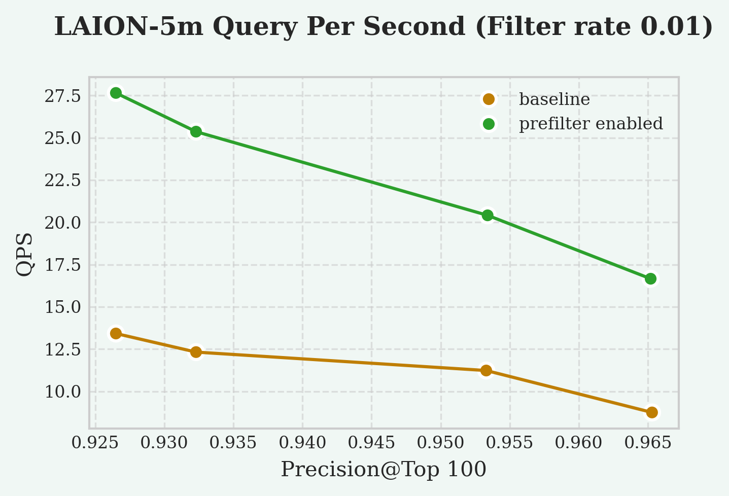
To retrieve $10$ vectors that satisfy the filter condition, the index returned approximately $970$ rows. This suggests that the index executed a large amount of redundant computation. If the index could leverage the filter condition for pruning, the computation would be significantly reduced. The vector index provides a GUC parameter vchordrq.prefilter that allows pruning of the search space based on the filter condition.

SET vchordrq.prefilter = on;

Prefilter enables the vector index to perform the search based on the filter. This prunes the search space, and a smaller search space leads to a more efficient search. However, checking whether the filter conditions are satisfied also introduces overhead. So prefilter is only recommended when the filter is strict (eliminating many rows) and cheap (computational cost is much lower than computing vector distances). To aid understanding, we present two incorrect usage examples:

• id % 97 > 0: this filter is relaxed
• email ~ '^([a-zA-Z]+)*$': this filter is expensive

Based on our experimental results, the QPS speedup at different selectivity is as follows:

• 200% speedup at 1% selectivity
• 5% speedup at 10% selectivity

Reference

This feature is not supported by vchordg.

Search Parameters (vchordrq)

vchordrq.prefilter

• Description: The vchordrq.prefilter GUC parameter enables condition evaluation before distance computation. For example, in the query SELECT * FROM items WHERE id % 2 = 0 ORDER BY embedding <-> '[3,1,2]' LIMIT 5, the index normally computes all useful embedding <-> '[3,1,2]' distances first and then pass the rows to PostgreSQL, which filters out rows where id % 2 != 0. This parameter allows the index to pre-evaluate the condition and discard non-matching rows before computing their distances, improving query efficiency.
• Type: boolean
• Default: false

12 - Prefetch

Prefetch dramatically accelerates queries that involve I/O operations. It works by proactively reading buffers into operating system page cache or PostgreSQL’s buffer pool based on the actual needs of the index.

Prefetch helps overlap I/O with computation, as well as I/O with other I/O operations, significantly reducing the time spent waiting for buffers during query execution, thereby improving overall query performance.

Prior to version 0.4.0, VectorChord used PostgreSQL’s synchronous I/O interface. Since then, VectorChord utilizes asynchronous I/O interface on newer versions of PostgreSQL. The I/O interface used by VectorChord can be controlled via GUC parameters.

In the GUC parameters, the synchronous I/O interface is referred to as read_buffer, the asynchronous I/O interface as read_stream, and VectorChord’s simulated asynchronous interface as prefetch_buffer.

For indexes much smaller than the memory, there is almost no difference among the three prefetch modes. read_stream accelerates all disk-based indexes; however, it is only available on PostgreSQL 17 and 18. To address this, VectorChord provides a simulated asynchronous I/O interface called prefetch_buffer, which is available on all PostgreSQL versions as a fallback for older versions. prefetch_buffer is less effective than read_stream.

To fully leverage this feature with read_stream, you need to enable asynchronous I/O on PostgreSQL 18. See also PostgreSQL Tuning.

Reference

Search Parameters (vchordrq)

vchordrq.io_search

• Description: This GUC parameter controls the I/O prefetching strategy for reading bit vectors in vector search, which can impact search performance on disk-based vectors.
• Type: string
• Domain: Depends on PostgreSQL version
  • PostgreSQL 13, 14, 15, 16: {"read_buffer", "prefetch_buffer"}
  • PostgreSQL 17, 18: {"read_buffer", "prefetch_buffer", "read_stream"}
• Default: Depends on PostgreSQL version
  • PostgreSQL 13, 14, 15, 16: prefetch_buffer
  • PostgreSQL 17, 18: read_stream
• Note:
  • read_buffer indicates a preference for ReadBuffer.
  • prefetch_buffer indicates a preference for both PrefetchBuffer and ReadBuffer.
  • read_stream indicates a preference for read_stream.

vchordrq.io_rerank

• Description: This GUC parameter controls the I/O prefetching strategy for reading full precision vectors in vector search, which can significantly impact search performance on disk-based vectors.
• Type: string
• Domain: Depends on PostgreSQL version
  • PostgreSQL 13, 14, 15, 16: {"read_buffer", "prefetch_buffer"}
  • PostgreSQL 17, 18: {"read_buffer", "prefetch_buffer", "read_stream"}
• Default: Depends on PostgreSQL version
  • PostgreSQL 13, 14, 15, 16: prefetch_buffer
  • PostgreSQL 17, 18: read_stream
• Note:
  • read_buffer indicates a preference for ReadBuffer.
  • prefetch_buffer indicates a preference for both PrefetchBuffer and ReadBuffer.
  • read_stream indicates a preference for read_stream.

Search Parameters (vchordg)

vchordg.io_search

• Description: This GUC parameter controls the I/O prefetching strategy for reading bit vectors in vector search, which can impact search performance on disk-based vectors.
• Type: string
• Domain: Depends on PostgreSQL version
  • PostgreSQL 13, 14, 15, 16: {"read_buffer", "prefetch_buffer"}
  • PostgreSQL 17, 18: {"read_buffer", "prefetch_buffer", "read_stream"}
• Default: Depends on PostgreSQL version
  • PostgreSQL 13, 14, 15, 16: prefetch_buffer
  • PostgreSQL 17, 18: read_stream
• Note:
  • read_buffer indicates a preference for ReadBuffer.
  • prefetch_buffer indicates a preference for both PrefetchBuffer and ReadBuffer.
  • read_stream indicates a preference for read_stream.

vchordg.io_rerank

• Description: This GUC parameter controls the I/O prefetching strategy for reading full precision vectors in vector search, which can significantly impact search performance on disk-based vectors.
• Type: string
• Domain: Depends on PostgreSQL version
  • PostgreSQL 13, 14, 15, 16: {"read_buffer", "prefetch_buffer"}
  • PostgreSQL 17, 18: {"read_buffer", "prefetch_buffer", "read_stream"}
• Default: Depends on PostgreSQL version
  • PostgreSQL 13, 14, 15, 16: prefetch_buffer
  • PostgreSQL 17, 18: read_stream
• Note:
  • read_buffer indicates a preference for ReadBuffer.
  • prefetch_buffer indicates a preference for both PrefetchBuffer and ReadBuffer.
  • read_stream indicates a preference for read_stream.

13 - Rerank in Table

PostgreSQL indexes store row identifiers and the values of the indexed columns. Typically, indexed columns have simple data types, for example, integers or strings with short length limits.

However, if the indexed column is of a vector type, both the table and the index store vectors, which means you pay twice the storage cost for the vectors. If you would like to reduce this cost, you can enable rerank_in_table when building the index. The index will then use a tricky approach where it does not store the vectors itself but reads them from the table when needed.

CREATE INDEX ON items USING vchordrq (embedding vector_l2_ops) WITH (options = $$
rerank_in_table = true
residual_quantization = true
$$);

Enabling this option results in degraded query performance and prefetch does not work when rerank_in_table is enabled.

It’s a trade-off of time for space, which is generally not recommended, so it’s intended only to address the specific issue of excessively high storage usage.

Reference

This feature is not supported by vchordg.

Indexing Options (vchordrq)

rerank_in_table

• Description: This option determines whether the vectors are fetched from the table. If so, the index will require less storage, but the query latency will increase significantly. It should only be enabled when disk space is extremely limited.
• Type: boolean
• Default: false
• Example:
  • rerank_in_table = false means that vectors are stored in both the index and the table, and fetched from the index in search.
  • rerank_in_table = true means that vectors are stored in the table only, and fetched from the table in search.

14 - Partitioning Tuning

For large tables, the partitioning phase dominates both build time and memory consumption.

Time complexity of partitioning is $O(FC^{2}DL)$, and the memory consumption in bytes can be approximated by $4DC(F + T + 1)$,

where:

• $D$ is the vector dimension, or build.internal.kmeans_dimension if set.
• $F$ is build.internal.sampling_factor.
• $C$ is build.internal.lists[-1].
• $T$ is build.internal.build_threads.
• $L$ is build.internal.kmeans_iterations.

This page introduces some tuning techniques to improve build time and memory consumption.

Hierarchical K-means

Hierarchical K-means is an algorithm that is faster than Lloyd’s algorithm. When applied this algorithm, the asymptotic time complexity is reduced to $O(FC^{1.5}DL)$. As a trade-off, it has a slight negative impact on search performance and recall.

Usage:

build.internal.kmeans_algorithm.hierarchical = {}

Reduce Sampling Factor

Reducing sampling factor improves build time and memory consumption linearly. As a trade-off, it has a moderate negative impact on search performance and recall.

Usage:

build.internal.sampling_factor = 64

Dimensionality reduction

Dimensionality reduction uses the fast Johnson–Lindenstrauss transform, reducing the dimensionality of the vectors involved in clustering to below their original dimension, thereby improving build time and memory consumption linearly. As a trade-off, it has a slight negative impact on search performance and recall.

Usage:

build.internal.kmeans_dimension = 100

Reference settings

LAION 100M

Dataset:

• Source: https://sisap-challenges.github.io/2024/datasets/
• Metric: Inner Product
• Dimension: 768
• Number of vectors: 100,000,000
• Number of test vectors: 1,000

Test machine (AWS EC2 i7i.4xlarge):

• CPU: Intel Xeon Platinum 8559C
• Number of vCPUs: 16
• Memory: 128 GiB
• Storage: 3750 GiB NVMe SSD

CREATE INDEX ON laion USING vchordrq (embedding vector_ip_ops) WITH (options = $$
build.pin = 2
build.internal.lists = [400, 160000]
build.internal.build_threads = 16
build.internal.spherical_centroids = true
build.internal.kmeans_algorithm.hierarchical = {}
build.internal.kmeans_dimension = 100
build.internal.sampling_factor = 64
$$);

Result:

• Total Build Time: 18 minutes
• Peak Memory: 6 GiB
• Test Case 1
  • Parameters
    • vchordrq.probes = '40,140'
    • vchordrq.epsilon = 1.4
  • QPS @ Top10: 120
  • Recall @ Top10: 0.949

DEEP 1B

Dataset:

• Source: https://big-ann-benchmarks.com/neurips21.html
• Metric: Euclidean
• Dimension: 96
• Number of vectors: 1,000,000,000
• Number of test vectors: 10,000

Test machine (AWS EC2 i7ie.6xlarge):

• CPU: Intel Xeon Platinum 8559C
• Number of vCPUs: 24
• Memory: 192 GiB
• Storage: 7500 GiB NVMe SSD

CREATE INDEX ON deep USING vchordrq (embedding vector_l2_ops) WITH (options = $$
build.pin = 2
residual_quantization = true
build.internal.lists = [800, 640000]
build.internal.build_threads = 24
build.internal.kmeans_algorithm.hierarchical = {}
$$);

Result:

• Total Build Time: 107 minutes
• Peak Memory: 64 GiB
• Test Case 1
  • Parameters
    • vchordrq.probes = '40,250'
  • QPS @ Top10: 68
  • Recall @ Top10: 0.951

15 - External Build

In addition to using the methods in Partitioning Tuning to achieve shorter build time and lower memory consumption at the cost of QPS and recall, you can also choose to run the partitioning phase offline on other machines or on GPUs. This feature is not supported by vchordg, since it does not have a partitioning phase.

Assume the table is t and the column to be indexed is val.

CREATE TABLE t (val vector(3));

Specifically, you need to sample the column for which the index will be built.

CREATE EXTENSION IF NOT EXISTS tsm_system_rows;
SELECT val FROM t TABLESAMPLE SYSTEM_ROWS(1000);

Based on these samples, you can partition the vector space into Voronoi cells. After that, you will create a table and insert your partitions.

CREATE TABLE public.t_build (id INTEGER NOT NULL UNIQUE, parent INTEGER, vector vector NOT NULL);
INSERT INTO public.t_build (id, parent, vector) VALUES (0, NULL, '{0.1, 0.2, 0.3}');
INSERT INTO public.t_build (id, parent, vector) VALUES (1, 0, '{0.1, 0.2, 0.3}');
INSERT INTO public.t_build (id, parent, vector) VALUES (2, 0, '{0.4, 0.5, 0.6}');
INSERT INTO public.t_build (id, parent, vector) VALUES (3, 0, '{0.7, 0.8, 0.9}');

The index can be created using the following syntax.

CREATE INDEX ON t USING vchordrq (embedding vector_l2_ops) WITH (options = $$
build.external.table = 'public.t_build'
$$);

Format

The table that stores the partition information must strictly follow the following schema:

• The first column must be id. Its type is integer. It must not be null. It must be unique.
• The second column must be parent. Its type is integer. It could not be null.
• The third column must be vector. Its type is vector. It must not be null. halfvec or other types are not supported yet.

Logically, this forms a tree. The distance from the root to each leaf must be the same.

If any of the above properties are not satisfied, an error will be reported.

Partitioning

To get started, here is a minimal code example for performing partitioning using faiss.

from typing import List
from faiss import Kmeans
import numpy

def partition(
    samples: List[numpy.Array[float]], lists: List[int]
) -> List[numpy.Array[float]]:
    dim = dataset.shape[1]
    results = []
    for i in range(len(lists) + 1):
        kmeans = Kmeans(
            dim,
            lists[len(lists) - 1 - i] if len(lists) - 1 - i >= 0 else 1,
            gpu=False,
            verbose=True,
            niter=10,
            seed=42,
            spherical=False,
        )
        kmeans.train(samples)
        results.push(kmeans.centroids)
        samples = kmeans.centroids
    return results

This computes the generators of all Voronoi cells across different levels. The parent-child relationships in the tree are determined by computing the shortest distances, but the details are omitted here. Any algorithm capable of generating multi-level Voronoi cells can be used, such as spherical K-means, balanced K-means or GPU K-means.