This is the multi-page printable view of this section. .
vchord Documentation
-
1: Getting Started
- 1.1: Overview
- 1.2: Installation
- 1.3: Vchord Suite
-
2: Usage
- 2.1: Indexing
- 2.2: Multi-Vector Retrieval
- 2.3: Graph Index
- 2.4: Quantization Types
- 2.5: Similarity Filter
- 2.6: PostgreSQL Tuning
- 2.7: Monitoring
- 2.8: Fallback Parameters
- 2.9: Measure Recall
- 2.10: Prewarm
- 2.11: Prefilter
- 2.12: Prefetch
- 2.13: Rerank in Table
- 2.14: Partitioning Tuning
- 2.15: External Build
- 3: Use Cases
- 4: Benchmarks
-
5: Administration
- 5.1: Migration
- 5.2: Scalability
- 5.3: Kubernetes
- 6: Customer Stories
Welcome to the vchord documentation. Select a topic below to get started with installation, indexing (vchordrq and vchordg), multi-vector retrieval, hybrid search, benchmarks, and production operations.
1 - Getting Started
1.1 - Overview
vchord is a PostgreSQL extension designed for scalable, high-performance, and disk-efficient vector similarity search.
With vchord, you can store 400,000 vectors for just $1, enabling significant savings: 6x more vectors compared to Pinecone’s optimized storage and 26x more than pgvector/pgvecto.rs for the same price1. For further insights, check out our launch blog post.
Features
vchord introduces remarkable enhancements over pgvecto.rs and pgvector:
⚡ Enhanced Performance: Delivering optimized operations with up to 5x faster queries, 16x higher insert throughput, and 16x quicker1 index building compared to pgvector’s HNSW implementation.
💰 Affordable Vector Search: Query 100M 768-dimensional vectors using just 32GB of memory, achieving 35ms P50 latency with top10 recall@95%, helping you keep infrastructure costs down while maintaining high search quality.
🔌 Seamless Integration: Fully compatible with pgvector data types and syntax while providing optimal defaults out of the box - no manual parameter tuning needed. Just drop in vchord for enhanced performance.
🔧 Accelerated Index Build: Leverage IVF to build indexes externally (e.g., on GPU) for faster KMeans clustering, combined with RaBitQ2 compression to efficiently store vectors while maintaining search quality through autonomous reranking.
📏 Long Vector Support: Store and search vectors up to 60,0003 dimensions, enabling the use of the best high-dimensional models like text-embedding-3-large with ease.
🌐 Scale As You Want: Based on horizontal expansion, the query of 5M / 100M 768-dimensional vectors can be easily scaled to 10000+ QPS with top10 recall@90% at a competitive cost4
Quick Start
For new users, we recommend using the Docker image to get started quickly. If you do not prefer Docker, please read installation guide for other installation methods.
In addition to the base image with the VectorChord extension, we provide an all-in-one image,
tensorchord/vchord-suite:pg18-latest. This comprehensive image includes all official TensorChord extensions. Developers should select an image tag that is compatible with their extension’s version, as indicated in the support matrix.
Then you can connect to the database using the psql command line tool. The default username is postgres, and the default password is mysecretpassword.
Now you can play with VectorChord!
VectorChord depends on pgvector, including the vector representation. Since you can use them directly, your application can be easily migrated without pain!
Similar to pgvector, you can create a table with vector column and insert some rows to it.
With VectorChord, you can create vchordrq indexes.
And then perform a vector search using SELECT ... ORDER BY ... LIMIT ....
For more usage, please read:
- Indexing
- Multi-Vector Retrieval
- Graph Index
- Quantization Types
- Similarity Filter
- PostgreSQL Tuning
- Monitoring
- Fallback Parameters
- Measure Recall
- Prewarm
- Prefilter
- Prefetch
- Rerank in Table
- Partitioning Tuning
- External Build
License
vchord is licensed under the GNU Affero General Public License v3.0 (AGPL-3.0-only). We welcome any commercial collaboration or support inquiries—please email us at rh@vonng.com with any questions.
-
Based on MyScale Benchmark with 768-dimensional vectors and 95% recall. Please check out our blog post for more details. ↩︎ ↩︎
-
Gao, Jianyang, and Cheng Long. “RaBitQ: Quantizing High-Dimensional Vectors with a Theoretical Error Bound for Approximate Nearest Neighbor Search.” Proceedings of the ACM on Management of Data 2.3 (2024): 1-27. ↩︎
-
There is a limitation at pgvector of 16,000 dimensions now. If you really have a large dimension(
16,000<dim<60,000), consider changing VECTOR_MAX_DIM and compile pgvector yourself. ↩︎ -
Please check our blog post for more details, the PostgreSQL scalability is powered by CloudNative-PG. ↩︎
1.2 - Installation
VectorChord is tested on the following operating system:
- Ubuntu (x86_64, aarch64)
- MacOS (x86_64, aarch64)
- Windows (x86_64)
- Alpine Linux (x86_64, aarch64) 1
- Debian (powerpc64le, s390x, riscv64) 2
Please report a bug if you encounter issues on any of the above operating systems, or submit a feature request for additional platform support.
Docker
VectorChord Image

The easiest way to try VectorChord is to run it from a ready-to use Docker image.
- Launch a VectorChord container in Docker.
- Connect to the database using the
psqlcommand line tool. The default username ispostgres.
- Run the following SQL to ensure the extension is enabled.
To achieve full performance, please mount the volume to PostgreSQL data directory by adding the option like:
-v $PWD/pgdata:/var/lib/postgresql/18/docker, on PostgreSQL 18-v $PWD/pgdata:/var/lib/postgresql/data, on PostgreSQL 14, 15, 16 and 17
You can configure PostgreSQL by the reference of the parent image in https://hub.docker.com/_/postgres/.
VectorChord Suite Image

In addition to the base image with the VectorChord extension, we provide an all-in-one image, tensorchord/vchord-suite:pg18-latest. This comprehensive image includes all official TensorChord extensions. Developers should select an image tag that is compatible with their extension’s version, as indicated in the support matrix.
- Launch a VectorChord container in Docker.
Other sections may align with the above.
VectorChord Scratch Image

We provide a scratch image that contains only the files of VectorChord. You can install VectorChord in any image using Docker’s COPY, like
This image can also be used as a CloudNativePG image volume extension. See also
Source
Build requirements:
- any port of
make clang >= 16withlibclangrust >= 1.93withcargo
It’s recommended to use Rustup for installing Rust on most platforms, while on Alpine Linux, using the system package manager is advised.
You can set the environment variable CC to specify the desired C compiler for the build system. If you do not set this variable, the build system automatically searches for clang and gcc. To compile all C code with clang, set CC to the path of clang. To compile all C code with gcc, set CC to the path of gcc; note that in this case, there is a requirement gcc >= 14.
Rust version requirement is not a long-term guarantee; we will raise the required Rust version with each new release.
These build requirements apply only to x86_64 and aarch64. For all other architectures, including powerpc64le, s390x and riscv64, nightly Rust and latest Clang are required.
If you have not installed PostgreSQL yet, please install PostgreSQL. If you have not installed pgvector yet, you could install pgvector before the 3rd step.
- Download the source code, build and install it with
make.
- Configure your PostgreSQL by modifying the
shared_preload_librariesto include the extension. And then restart the PostgreSQL cluster.
- Run the following SQL to ensure the extension is enabled.
Tuning
VectorChord performs runtime CPU dispatch for SIMD code. If you want the compiler to optimize the whole program for a particular CPU, you could instruct it to generate code for that CPU.
To see all valid CPU options and the default CPU for your target triple, run:
To generate code for the host machine, run:
Please note that binaries generated with a specific target-cpu are not compatible with other CPUs.
You can also do it by using Cargo’s configuration.
Debian
If you have not installed PostgreSQL yet, please install PostgreSQL following https://www.postgresql.org/download/linux/debian/. If you have not installed pgvector yet, you could install pgvector by apt install postgresql-18-pgvector before the 3rd step.
New VectorChord releases are hosted at github.com/pgsty/vchord/releases, while historical releases (1.1.1 and earlier) remain available at github.com/tensorchord/VectorChord/releases.
- Download Debian packages in the release page, and install them by
apt.
- Configure your PostgreSQL by modifying the
shared_preload_librariesto include the extension. And then restart the PostgreSQL cluster.
- Run the following SQL to ensure the extension is enabled.
Ubuntu
If you have not installed PostgreSQL yet, please install PostgreSQL following https://www.postgresql.org/download/linux/ubuntu/. If you have not installed pgvector yet, you could install pgvector by apt install postgresql-18-pgvector before the 3rd step.
New VectorChord releases are hosted at github.com/pgsty/vchord/releases, while historical releases (1.1.1 and earlier) remain available at github.com/tensorchord/VectorChord/releases.
- Download Debian packages in the release page, and install them by
apt.
- Configure your PostgreSQL by modifying the
shared_preload_librariesto include the extension. And then restart the PostgreSQL cluster.
- Run the following SQL to ensure the extension is enabled.
PGXN
See Source for build requirements.
If you have not installed PostgreSQL yet, please install PostgreSQL. If you have not installed pgvector yet, you could install pgvector by pgrxclient install vector before the 3rd step.
- Install VectorChord from PostgreSQL Extension Network with:
- Configure your PostgreSQL by modifying the
shared_preload_librariesto include the extension. And then restart the PostgreSQL cluster.
- Run the following SQL to ensure the extension is enabled.
There is a broken VectorChord 0.4.1 package on PGXN. Please do not use it. Use version 0.4.2 or later instead.
Prebuilt binaries
deprecatedPrebuilt binaries may not match the PostgreSQL in ABI on your machine, which could cause silent errors. We strongly recommend that you build from source in this case.
If you have not installed PostgreSQL yet, please install PostgreSQL. If you have not installed pgvector yet, you could install pgvector before the 3rd step.
- Download prebuilt binaries in the release page, and repackage it referring to your distribution’s documentation. Then install it by system package manager. We do not recommend doing this, but if you wish, you can also manually copy the files to the system directory.
- Configure your PostgreSQL by modifying the
shared_preload_librariesto include the extension. And then restart the PostgreSQL cluster.
- Run the following SQL to ensure the extension is enabled.
-
VectorChord is tested with PostgreSQL 15 in
communityrepository, 16 and 17 inmainrepository on Alpine Linux 3.22. ↩︎ -
VectorChord is tested with PostgreSQL 13, 14, 15, 16, 17 and 18 in PostgreSQL’s official repository on
powerpc64le, and PostgreSQL 15 and 17 in Debian’s official repository ons390xandriscv64, with QEMU user space emulator. ↩︎
1.3 - Vchord Suite
Retrieval-Augmented Generation (RAG) is revolutionizing our interaction with vast datasets and language models. RAG systems offer more precise, contextually aware, and current answers by retrieving pertinent information before generating responses. Nonetheless, constructing robust, scalable, and efficient RAG pipelines poses considerable challenges, particularly for production use.
Many solutions feature complex architectures, using distinct databases for vector search, keyword search, and primary data storage. This commonly results in data synchronization challenges, greater infrastructure complexity, and higher operational costs.
What if you could build a powerful, production-ready RAG system directly within your trusted PostgreSQL database?
Enter the Vchord Suite, a collection of PostgreSQL extensions designed to bring high-performance vector search, native BM25 ranking, and flexible tokenization capabilities right into Postgres. Let’s explore the components and how they enable next-generation RAG solutions.
What is the Vchord Suite?
The suite comprises three key PostgreSQL extensions working in concert:
-
vchord(pgsty/vchord): The core vector search engine. It’s specifically designed for scalable, high-performance, and disk-efficient vector similarity search within PostgreSQL. -
vchord_bm25(pgsty/vchord_bm25): This extension implements the sophisticated BM25 ranking algorithm directly inside PostgreSQL, leveraging efficient Block-WeakAnd algorithms. BM25 is a standard for relevance ranking based on keyword frequency and document characteristics. -
pg_tokenizer(pgsty/pg_tokenizer): Provides essential text tokenization capabilities needed for effective full-text search, enabling fine-grained control over how text is processed for full-text search.
By combining these extensions, you unlock powerful capabilities for building advanced RAG systems entirely within PostgreSQL.
How to Use the Vchord Suite
You can use the tensorchord/vchord-suite Docker image to run multiple extensions which are provided by TensorChord. The image is based on the Docker official PostgreSQL image and includes the following extensions:
vchordpg_tokenizervchord_bm25vector
Use Cases for the Vchord Suite
Use Case 1: Powerful Hybrid Search with Native BM25 and vchord
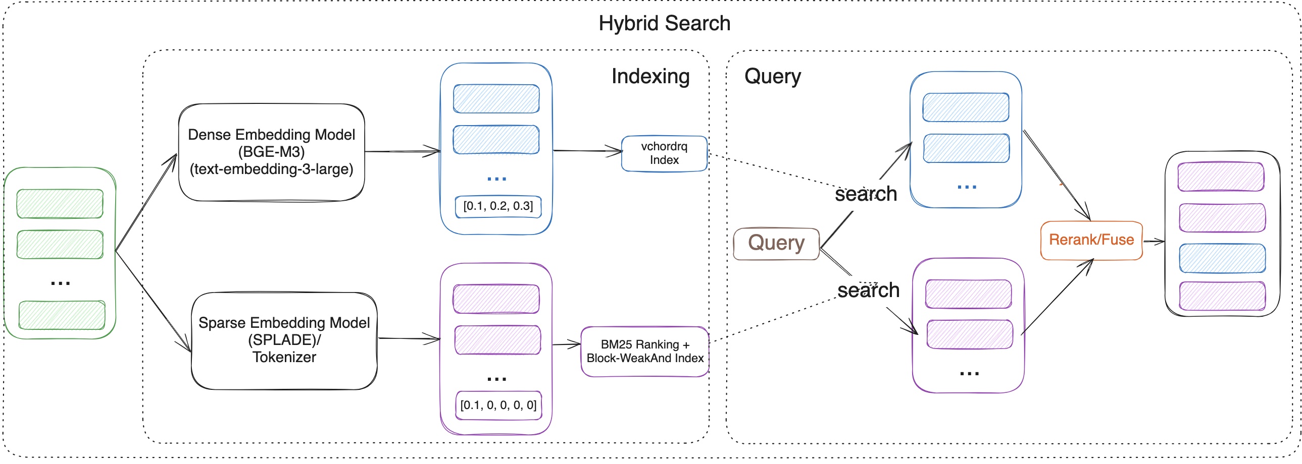
In the RAG era, effective retrieval is paramount. Neither keyword search nor vector search alone is perfect:
-
Keyword Search (like BM25): Excels at precision, finding documents with exact keyword matches. It’s great for structured queries and term-specific searches. However, it struggles with synonyms, paraphrasing, and understanding the underlying meaning or semantic intent. (Leverages
vchord_bm25andpg_tokenizer). -
Vector Search: Captures deep semantic meaning and relationships between concepts, allowing it to find relevant information even if the exact keywords aren’t present. However, it can sometimes lack precision for queries demanding specific term matches. (Leverages
vchord).
The Solution: Hybrid Search. By combining the strengths of both approaches within PostgreSQL, the Vchord Suite bridges this gap. You can run a query that leverages:
-
vchord_bm25(powered bypg_tokenizer) for keyword precision. -
vchordfor semantic understanding.
The results from both can be intelligently combined (e.g., using reciprocal rank fusion - RRF or Model-based rerank) to produce a final ranking that is more accurate, contextually relevant, and semantically aware than either method could achieve alone. This delivers significantly better retrieval performance for your RAG applications.
Use Case 2: Beyond Text - OCR-Free RAG with ColQwen2 & vchord
Building RAG systems for documents like PDFs or scanned images often involves cumbersome pre-processing pipelines. Traditional methods rely heavily on Optical Character Recognition (OCR) and layout analysis to extract text. This process can be:
-
Slow: OCR can be computationally expensive.
-
Error-Prone: OCR accuracy varies significantly depending on document quality.
-
Lossy: Crucial visual contexts like tables, figures, formatting, and relative positioning is often lost during text extraction.
The Solution: OCR-Free, Visually-Aware RAG. What if you could query documents based on how they look and their content, without explicit OCR?
This is now achievable by combining:
-
Multi-Modal Vision Language Models (VLMs): Models like ColQwen2 can process images (document pages) and generate embeddings that capture both textual content and visual layout information.
-
vchord’s Multi-Vector Capabilities:vchordcan efficiently store and search multiple vectors per document within PostgreSQL – allowing you to store embeddings representing different aspects (e.g., text content, visual layout).
With this setup, you can query your document database using prompts that reference visual elements (“Find documents with a bar chart comparing sales figures”) or combined textual and visual cues, directly within PostgreSQL. This simplifies your RAG stack, potentially boosts retrieval accuracy by preserving visual context, and eliminates the bottlenecks associated with traditional OCR pipelines.
Why Build RAG in PostgreSQL?
Leveraging the Vchord Suite within PostgreSQL offers significant advantages:
-
Unified Data: Keep your source data, text, metadata, and vector embeddings all in one place.
-
Reduced Complexity: Eliminate the need for separate vector databases and synchronization pipelines.
-
Leverage Existing Infrastructure: Utilize your existing PostgreSQL expertise, tooling, and operational practices.
-
Transactional Integrity: Benefit from PostgreSQL’s robust ACID compliance.
-
Rich Ecosystem: Access the wide array of tools and features available within the PostgreSQL ecosystem.
Conclusion
The Vchord Suite transforms PostgreSQL into a powerful, production-ready platform for building advanced RAG solutions. By integrating high-performance vector search (vchord), sophisticated keyword ranking (vchord_bm25), and flexible text processing (pg_tokenizer), you can implement cutting-edge techniques like hybrid search and OCR-free multi-modal retrieval directly within your database. Simplify your architecture, enhance retrieval accuracy, and unlock the full potential of RAG with Vchord in PostgreSQL.
Blog Posts
In our recent blog posts, we shared some user cases where all Docker images can be replaced with VectorChord Suite image.
References
2 - Usage
2.1 - Indexing
VectorChord’s index type vchordrq divides vectors into lists and searches only a subset of lists closest to the query vector. It provides fast build time and low memory consumption, while delivering significantly better performance than both hnsw and ivfflat.
Let’s start by creating a table named items with an embedding column of type vector(n), and then populate it with sample data.
To create a vchordrq index, you can use the following SQL.
After the index is built, you can perform a vector search using it to retrieve the nearest neighbors to a vector.
You can also add filters to vector search queries as needed.
Tuning
When there are less than rows in the table, you usually don’t need to set the index options.
However, as the number of rows grows, partitioning becomes necessary and can be configured using index options. options are specified using a TOML: Tom’s Obvious Minimal Language string. You can refer to #Index Options for more information.
The parameter lists should be tuned based on the number of rows. The following table provides guidelines for choosing an appropriate value. When querying, choose vchordrq.probes accordingly.
| Number of Rows | Recommended Number of Partitions | Example lists |
|---|---|---|
| N/A | [] |
|
[2000] |
||
[10000] |
||
[80000] |
The process of building an index involves two steps: partitioning the vector space first, and then inserting rows into the index. The first step, partitioning the vector space, can be sped up using multiple threads.
The second step, inserting rows, can be parallelized using multiple processes. Refer to PostgreSQL Tuning.
For most datasets using cosine similarity, enabling residual_quantization and build.internal.spherical_centroids improves both QPS and recall.
To improve the build speed, you may opt to use more shared memory to accelerate the process by setting build.pin to 2.
For large tables, time and memory overhead are dominated by the partitioning phase. See Partitioning Tuning for further tuning.
You can also refer to External Build to offload the partitioning phase to other machines.
Reference
Operator Classes (vchordrq)
vchordrq
The following table lists all available operator classes supported by vchordrq.
| Operator Class | Description | Operator 1 | Operator 2 |
|---|---|---|---|
vector_l2_ops |
index works for vector type and Euclidean distance |
<->(vector,vector) |
<<->>(vector,vector) |
vector_ip_ops |
index works for vector type and negative inner product |
<#>(vector,vector) |
<<#>>(vector,vector) |
vector_cosine_ops |
index works for vector type and cosine distance |
<=>(vector,vector) |
<<=>>(vector,vector) |
halfvec_l2_ops |
index works for halfvec type and Euclidean distance |
<->(halfvec,halfvec) |
<<->>(halfvec,halfvec) |
halfvec_ip_ops |
index works for halfvec type and negative inner product |
<#>(halfvec,halfvec) |
<<#>>(halfvec,halfvec) |
halfvec_cosine_ops |
index works for halfvec type and cosine distance |
<=>(halfvec,halfvec) |
<<=>>(halfvec,halfvec) |
rabitq8_l2_ops |
index works for rabitq8 type and Euclidean distance |
<->(rabitq8,rabitq8) |
<<->>(rabitq8,rabitq8) |
rabitq8_ip_ops |
index works for rabitq8 type and negative inner product |
<#>(rabitq8,rabitq8) |
<<#>>(rabitq8,rabitq8) |
rabitq8_cosine_ops |
index works for rabitq8 type and cosine distance |
<=>(rabitq8,rabitq8) |
<<=>>(rabitq8,rabitq8) |
rabitq4_l2_ops |
index works for rabitq4 type and Euclidean distance |
<->(rabitq4,rabitq4) |
<<->>(rabitq4,rabitq4) |
rabitq4_ip_ops |
index works for rabitq4 type and negative inner product |
<#>(rabitq4,rabitq4) |
<<#>>(rabitq4,rabitq4) |
rabitq4_cosine_ops |
index works for rabitq4 type and cosine distance |
<=>(rabitq4,rabitq4) |
<<=>>(rabitq4,rabitq4) |
vector_maxsim_ops |
index works for vector[] type and scalable vector-similarity |
@#(vector[],vector[]) |
N/A |
halfvec_maxsim_ops |
index works for halfvec[] type and scalable vector-similarity |
@#(halfvec[],halfvec[]) |
N/A |
rabitq8_maxsim_ops |
index works for rabitq8[] type and scalable vector-similarity |
@#(rabitq8[],rabitq8[]) |
N/A |
rabitq4_maxsim_ops |
index works for rabitq4[] type and scalable vector-similarity |
@#(rabitq4[],rabitq4[]) |
N/A |
<->, <#> and <=> are operators defined by pgvector.
| Name | Description |
|---|---|
<-> |
squared Euclidean distance |
<#> |
negative dot product |
<=> |
cosine distance |
<<->>, <<#>>, <<=>> are operators defined by VectorChord. For more information about <<->>, <<#>>, <<=>>, refer to Similarity Filter.
@# is an operator defined by VectorChord. For more information about @#, refer to Multi-Vector Retrieval.
rabitq8, rabitq4 are types defined by VectorChord. For more information about rabitq8, rabitq4, refer to Quantization Types.
The operator classes for MaxSim are available since version 0.3.0. The operator classes for rabitq8 and rabitq4 are available since version 1.1.0.
Indexing Options (vchordrq)
vchordrq
residual_quantization
- Description: This option determines whether residual quantization is used. If you are not familiar with residual quantization, you can read this blog for more information. In short, residual quantization is a technique that improves the accuracy of vector search by quantizing the residuals of the vectors.
- Type: boolean
- Default:
false - Example:
residual_quantization = falsemeans that residual quantization is not used.residual_quantization = truemeans that residual quantization is used.
- Note: This option is not supported for
rabitq8andrabitq4.
degree_of_parallelism
since v1.0.0
- Description: This option is a hint that specifies the degree of parallelism. In most cases, you do not need to change it. If you are using a CPU with more than
32threads and wish to utilize more threads for PostgreSQL, you may set it to the number of threads for better performance. - Type: integer
- Default:
32 - Domain:
[1, 256] - Example:
degree_of_parallelism = 32hints to the index that32or less processes may access on the index concurrently.degree_of_parallelism = 64hints to the index that64or less processes may access on the index concurrently.
build.pin
since v0.2.1
- Description: This option determines whether shared memory is used for indexing. For large tables, you can choose to enable this option to speed up the build process.
- Type: union of integer and boolean
- Default:
-1since v1.0.0falseuntil v0.5.3
- Domain:
{-1, 0, 1, 2, false, true}since v1.0.0{false, true}until v0.5.3
- Example:
build.pin = 2means the hot portion of the index is cached in memory.build.pin = 1means a subset of the hot portion of the index is cached in memory, consuming less memory.build.pin = 0means that this feature is enabled but nothing is actually cached. This option is for debugging purposes only.build.pin = -1means that this feature is disabled.build.pin = falseis the legacy form ofbuild.pin = -1.build.pin = trueis the legacy form ofbuild.pin = 1.
Default Build Options
since v0.5.3This is the default value of index building. The index will not be partitioned. In terms of semantics, build.default = {} is similar to build.internal.lists = [].
Internal Build Options (vchordrq)
vchordrq
build.internal.lists
- Description: This option determines the hierarchical structure of the vector space partitioning.
- Type: list of integers
- Default:
[]since v0.3.0[1000]until v0.2.2: implicit behavior is not ideal
- Example:
build.internal.lists = []means that the vector space is not partitioned.build.internal.lists = [4096]means the vector space is divided into cells.build.internal.lists = [4096, 262144]means the vector space is divided into cells, and those cells are further divided into smaller cells.
- Note: The index partitions the vector space into multiple Voronoi cells based on centroids, iteratively creating a hierarchical space partition tree. Each leaf node in this tree represents a region with an associated list storing vectors in that region. During insertion, vectors are placed in lists corresponding to their appropriate leaf nodes. For queries, the index optimizes search by excluding lists whose leaf nodes are distant from the query vector, effectively pruning the search space. If the length of
listsis , thelistsoption should be no less than , where is the number of vectors in the table.
build.internal.spherical_centroids
- Description: This option determines whether to perform spherical K-means – the centroids are L2 normalized after each iteration, you can refer to option
sphericalin here. - Type: boolean
- Default:
false - Example:
build.internal.spherical_centroids = falsemeans that spherical k-means is not performed.build.internal.spherical_centroids = truemeans that spherical k-means is performed.
- Note: Set this to
trueif your model generates embeddings that use cosine similarity as the metric.
build.internal.sampling_factor
since v0.2.0
- Description: This option determines the number of vectors the K-means algorithm samples per cluster. The higher this value, the slower the build, the greater the memory consumption in building, and the better search performance.
- Type: integer
- Domain:
[0, 1024] - Default:
256 - Example:
build.internal.sampling_factor = 256means that the K-means algorithm samples vectors, where is the maximum value inbuild.internal.lists.build.internal.sampling_factor = 32means that the K-means algorithm samples vectors, where is the maximum value inbuild.internal.lists. This reduces K-means’ time and memory usage to approximately of what it would be with the default value of256.
build.internal.kmeans_iterations
since v0.2.2
- Description: This option determines the number of iterations for K-means algorithm. The higher this value, the slower the build.
- Type: integer
- Domain:
[0, 1024] - Default:
10 - Example:
build.internal.kmeans_iterations = 10means that the K-means algorithm performs iterations.build.internal.kmeans_iterations = 100means that the K-means algorithm performs iterations.
build.internal.build_threads
- Description: This option determines the number of threads used by K-means algorithm. The higher this value, the faster the build, and greater load on the server in building.
- Type: integer
- Domain:
[1, 255] - Default:
1 - Example:
build.internal.build_threads = 1means that the K-means algorithm uses thread.build.internal.build_threads = 4means that the K-means algorithm uses threads.
build.internal.kmeans_algorithm
since v1.0.0
- Description: This option determines the K-means algorithm to be used.
- Type: object
- Example:
build.internal.kmeans_algorithm.lloyd = {}. This uses Lloyd’s algorithm. This is the default value.build.internal.kmeans_algorithm.hierarchical = {}. This uses hierarchical clustering. Compared to Lloyd’s algorithm, this approach is much faster, but it may cause a loss of accuracy.
build.internal.kmeans_dimension
since v1.0.0
- Description: This option determines the dimension to use for K-means input and output. This feature employs dimensionality reduction and expansion via resampling, effectively reducing K-means’ time and memory consumption, but it may cause a loss of accuracy.
- Type: union of integer and null
- Default: null
- Example:
- If this option is not set, this feature is disabled.
build.internal.kmeans_dimension = 100means that K-means will process vectors with dimensions. For original vectors of dimensions, this reduces K-means’ time and memory usage to approximately of what it would be without this feature.
Search Parameters (vchordrq)
vchordrq
vchordrq.enable_scan
since v0.5.0
- Description: Enables or disables the query planner’s use of
vchordrqindex scan. It’s for testing purposes. - Type: boolean
- Default:
on - Example:
vchordrq.enable_scan = offdisables the query planner’s use ofvchordrqindex scan.vchordrq.enable_scan = onenables the query planner’s use ofvchordrqindex scan.
vchordrq.probes
- Description: This GUC parameter
vchordrq.probescontrols how the vector space assists in query pruning. The more probes, the more accurate the search, but also the slower it is. - Type: list of integers
- Default:
10until v0.2.2: the default value was 10 before `lists` defaulted to empty- This parameter supports fallback.
- Example:
SET vchordrq.probes = 1means that only one probe is used.SET vchordrq.probes = 10means that ten probes are used.
- Note: The default value is an empty list. The length of this option must match the length of
lists.- If
lists = [], then probes must be - If
lists = [11, 22], then probes can be2,4or4,8. It must not be incorrectly shaped, for example,3,7,8,9,5,5,5,5.
- If
vchordrq.epsilon
- Description: Even after pruning, the number of retrieved vectors remains substantial. The index employs the RaBitQ algorithm to quantize vectors into bit vectors, which require just the memory of single-precision floating-point vectors. Most computations are integer-based, leading to faster processing. Unlike conventional quantization algorithms, RaBitQ estimates not only distances but also their lower bounds. The index computes the lower bound for each vector and dynamically adjusts the number of vectors needing recalculated distances, based on the query count, thus balancing performance and accuracy. The GUC parameter
vchordrq.epsiloncontrols the conservativeness of the lower bounds of distances. The higher the value, the higher the accuracy, but the worse the performance. The default value tends to favor higher accuracy than needed for most use cases, so you can try lowering this parameter to achieve better performance. - Type: real
- Default:
1.9- This parameter supports fallback.
- Domain:
[0.0, 4.0] - Example:
SET vchordrq.epsilon = 0.1indicates you are using a very optimistic lower bound estimation. You set it this way because your dataset is not sensitive to the lower bound estimation, for the precision you need.SET vchordrq.epsilon = 4.0indicates you are using a very pessimistic lower bound estimation. You set it this way because your dataset is not very sensitive to the lower bound estimation, for the precision you need.
vchordrq.prewarm_dim
removed in v0.4.0
- Description: The
vchordrq.prewarm_dimGUC parameter is used to precompute the RaBitQ projection matrix for the specified dimensions. This can help to reduce the latency of the first query after the PostgreSQL cluster is started. - Type: list of integers
- Default:
64,128,256,384,512,768,1024,1536 - Example:
ALTER SYSTEM SET vchordrq.prewarm_dim = '64,128'means that the projection matrix will be precomputed for dimensions 64 and 128.
- Note:
- This setting requires a database restart to take effect.
- Since
v0.4.0, a new algorithm made this option obsolete.
vchordrq.max_scan_tuples
since v0.2.0
- Description: The GUC parameter
vchordrq.max_scan_tuplescontrols the maximum number of tuples that can be scanned in a vector search. In most cases, you do not need to set this parameter, because theLIMITclause serves a similar purpose. However, when aWHEREclause is present, theLIMITclause applies after filtering, while this GUC parameter applies before filtering. This parameter is intended to prevent performance degradation when the filtering selectivity is very low. - Type: integer
- Default:
-1 - Domain:
[-1, 2147483647] - Example:
SET vchordrq.max_scan_tuples = 999indicates the index scan returns at most tuples.SET vchordrq.max_scan_tuples = -1indicates no limit on the number of tuples.
- Note: This parameter has no effect when set to
-1.
2.2 - Multi-Vector Retrieval
Multi-Vector Retrieval is an advanced technique used in Retrieval-Augmented Generation (RAG) systems to enhance document retrieval by leveraging multiple vectors per document.
Unlike Single-Vector Retrieval, Multi-Vector Retrieval using the MaxSim operator enables capturing fine-grained semantic relationships.
Refer to our blog for more details on building an end-to-end Multi-Vector Retrieval application.
How to start
Late interaction models embed documents and queries as vector arrays separately and compute similarity through an operator called MaxSim. The definition of the MaxSim operator is , meaning that for each vector in the query vector array, the closest vector in the document vector array is found, their dot product is calculated, and the results are summed.
In VectorChord, the symbol for this operator is @#. The left operand is the document vector array, and the right operand is the query vector array. While the original MaxSim operator is similarity-based, while the operator in VectorChord is based on distance. VectorChord’s implementation interprets it as a distance metric by negating the similarity score.
To construct an index for vector arrays, first create a table named items with a column named embeddings of type vector(n)[]. Then, populate the table with generated data.
Queries using the MaxSim operator can be accelerated with indexing, like other vector operators.
Then you can perform a vector search with the index.
Reference
This feature is not supported by vchordg.
Operator Classes
Refer to
Search Parameters (vchordrq)
vchordrq
The indexing mechanism for MaxSim operators works similarly to other vector operators. When an index is built on a column of vector arrays, each vector within the arrays is individually inserted into the index data structure. During querying, the index performs a separate vector search for each vector in the query array. By default, the index does not rerank the results. Instead, it uses RaBitQ’s estimated distances as a substitute for actual distances. The index then merges the results from all separated vector searches to produce the final output.
There are a few extra parameters used by maxsim indexes.
vchordrq.maxsim_refine
since v0.3.0
- Description: This GUC parameter
vchordrq.maxsim_refinemakes the index rerank the results, replacing RaBitQ’s estimated distances with actual distances, until the distances of the top-k nearest vectors have all been recalculated. - Type: integer
- Domain:
[0, 2147483647] - Default:
0- This parameter supports fallback.
- Example:
SET vchordrq.maxsim_refine = 0means that the index always uses RaBitQ’s estimated distances.SET vchordrq.maxsim_refine = 1024means that the index reranks the results, replacing RaBitQ’s estimated distances with actual distances, until the distances of the top-1024 nearest vectors have all been recalculated.
vchordrq.maxsim_threshold
since v0.3.0
- Description: This GUC parameter
vchordrq.maxsim_thresholdenables more aggressive estimation of missing values. With this setting, the index identifies the first cluster in the lowest-level lists whose cumulative size meets or exceedsvchordrq.maxsim_threshold, and uses its distance to the query vector for estimating the missing values. - Type: integer
- Domain:
[0, 2147483647] - Default:
0- This parameter supports fallback.
- Example:
SET vchordrq.maxsim_threshold = 0means that the more aggressive estimation strategy is not enabled.SET vchordrq.maxsim_threshold = 1024means that the index identifies the first cluster in the lowest-level lists whose cumulative size meets or exceeds1024, and uses its distance to the query vector for estimating the missing values.
2.3 - Graph Index
VectorChord’s index type vchordg is a disk-based graph index. It has low memory consumption.
Let’s start by creating a table named items with an embedding column of type vector(n), and then populate it with sample data.
To create a vchordg index, you can use the following SQL.
This feature is in preview.
Tuning
When building an index, two options usually need tuning: m and ef_construction. m is the maximum number of neighbors per vertex, and ef_construction is the size of the dynamic list containing the nearest neighbors during insertion.
In search, you need to tune ef_search. ef_search is the size of the dynamic list containing the nearest neighbors during search.
As a disk-based index, vchordg usually requires only the quantized vectors to be kept in the buffer pool to maintain performance. By default, vchordg quantizes a -dimensional vector to bits. Let the number of rows be . Then, the total memory required for the index is bits. If you have very limited memory and are using ultra-high dimensional vectors, consider quantizing a vector to bits. Then, the total memory required for the index is bits.
The index building can be sped up by using multiple processes. Refer to PostgreSQL Tuning.
Reference
Operator Classes (vchordg)
vchordg
The following table lists all available operator classes supported by vchordg.
| Operator Class | Description | Operator 1 | Operator 2 |
|---|---|---|---|
vector_l2_ops |
index works for vector type and Euclidean distance |
<->(vector,vector) |
<<->>(vector,vector) |
vector_ip_ops |
index works for vector type and negative inner product |
<#>(vector,vector) |
<<#>>(vector,vector) |
vector_cosine_ops |
index works for vector type and cosine distance |
<=>(vector,vector) |
<<=>>(vector,vector) |
halfvec_l2_ops |
index works for halfvec type and Euclidean distance |
<->(halfvec,halfvec) |
<<->>(halfvec,halfvec) |
halfvec_ip_ops |
index works for halfvec type and negative inner product |
<#>(halfvec,halfvec) |
<<#>>(halfvec,halfvec) |
halfvec_cosine_ops |
index works for halfvec type and cosine distance |
<=>(halfvec,halfvec) |
<<=>>(halfvec,halfvec) |
rabitq8_l2_ops |
index works for rabitq8 type and Euclidean distance |
<->(rabitq8,rabitq8) |
<<->>(rabitq8,rabitq8) |
rabitq8_ip_ops |
index works for rabitq8 type and negative inner product |
<#>(rabitq8,rabitq8) |
<<#>>(rabitq8,rabitq8) |
rabitq8_cosine_ops |
index works for rabitq8 type and cosine distance |
<=>(rabitq8,rabitq8) |
<<=>>(rabitq8,rabitq8) |
rabitq4_l2_ops |
index works for rabitq4 type and Euclidean distance |
<->(rabitq4,rabitq4) |
<<->>(rabitq4,rabitq4) |
rabitq4_ip_ops |
index works for rabitq4 type and negative inner product |
<#>(rabitq4,rabitq4) |
<<#>>(rabitq4,rabitq4) |
rabitq4_cosine_ops |
index works for rabitq4 type and cosine distance |
<=>(rabitq4,rabitq4) |
<<=>>(rabitq4,rabitq4) |
<<->>, <<#>>, <<=>> are operators defined by VectorChord. For more information about <<->>, <<#>>, <<=>>, refer to Similarity Filter.
rabitq8, rabitq4 are types defined by VectorChord. For more information about rabitq8, rabitq4, refer to Quantization Types.
The first 6 operator classes are available since version 0.5.0, and the last 6 operator classes are available since version 1.1.0.
Indexing Options (vchordg)
vchordg
bits
since v0.5.0
- Description: The ratio of bits to dimensions after RaBitQ quantization.
bits = 2provides better recall and QPS, whilebits = 1consumes less memory. - Type: integer
- Default:
2 - Example:
bits = 2means a -dimensional vector is quantized to bits.bits = 1means a -dimensional vector is quantized to bits .
m
since v0.5.0
- Description: The maximum number of neighbors per vertex. The larger
mis, the better the performance, but the higher the storage requirement.mcorresponds to in HNSW and in DiskANN. - Type: integer
- Default:
32 - Example:
m = 32means that there are at most neighbors per vertex.m = 64means that there are at most neighbors per vertex.
ef_construction
since v0.5.0
- Description: The size of the dynamic list containing the nearest neighbors during insertion. The larger
ef_constructionis, the better the performance, but the slower the insertion.ef_constructioncorresponds to in HNSW and in DiskANN. - Type: integer
- Default:
64 - Example:
ef_construction = 64means that the size of the dynamic list containing the nearest neighbors is during insertion.ef_construction = 128means that the size of the dynamic list containing the nearest neighbors is during insertion.
alpha
since v0.5.0
- Description: The
alphavalues selected during pruning.alphacorresponds to in DiskANN. This option must be an ascending list, where the first element is1.0and the last element is less than2.0. - Type: list of floats
- Default:
[1.0, 1.2] - Example:
alpha = [1.0, 1.2]is equivalent to settingalpha = 1.2in DiskANN.alpha = [1.0]is equivalent to the default pruning strategy in HNSW.
- Note: this option is ineffective when the distance metric is negative inner product.
beam_construction
since v0.5.0
- Description: Beam width used during insertion. Beam width refers to the number of vertices accessed at once. Since the time to randomly read a small number of sectors from the SSD is almost the same as reading a single sector, a larger beam width effectively reduces the number of round trips to the SSD, resulting in better performance. Since it increases computation, it is disadvantageous for indexes that fit entirely in memory.
- Type: integer
- Default:
1 - Example:
beam_construction = 8means that the index accesses 8 vertices at once during insertion.beam_construction = 1means that the index accesses 1 vertex at once during insertion.
Search Parameters (vchordg)
vchordg
vchordg.enable_scan
since v0.5.0
- Description: Enables or disables the query planner’s use of
vchordgindex scan. It’s for testing purposes. - Type: boolean
- Default:
on - Example:
vchordg.enable_scan = offdisables the query planner’s use ofvchordgindex scan.vchordg.enable_scan = onenables the query planner’s use ofvchordgindex scan.
vchordg.ef_search
since v0.5.0
- Description: The size of the dynamic list containing the nearest neighbors in search. The larger
vchordg.ef_searchis, the better the recall, but the worse the QPS.vchordg.ef_searchcorresponds to in HNSW and DiskANN. - Type: integer
- Default:
64- This parameter supports fallback.
- Domain:
[1, 65535] - Example:
SET vchordg.ef_search = 64indicates the size of the dynamic list containing the nearest neighbors is during search.SET vchordg.ef_search = 128indicates the size of the dynamic list containing the nearest neighbors is during search.
vchordg.beam_search
since v0.5.0
- Description: Beam widths used during search. Beam width refers to the number of vertices accessed at once. Since the time to randomly read a small number of sectors from the SSD is almost the same as reading a single sector, a larger beam width effectively reduces the number of round trips to the SSD, resulting in better performance. Since it increases computation, it is disadvantageous for indexes that fit entirely in memory.
- Type: integer
- Default:
1 - Domain:
[1, 65535] - Example:
SET vchordg.beam_search = 8indicates that the index accesses 8 vertices at once during search.SET vchordg.beam_search = 1indicates that the index accesses 1 vertex at once during search.
vchordg.max_scan_tuples
since v0.5.0
- Description: The GUC parameter
vchordg.max_scan_tuplescontrols the maximum number of tuples that can be scanned in a vector search. In most cases, you do not need to set this parameter, because theLIMITclause serves a similar purpose. However, when aWHEREclause is present, theLIMITclause applies after filtering, while this GUC parameter applies before filtering. This parameter is intended to prevent performance degradation when the filtering selectivity is very low. - Type: integer
- Default:
-1 - Domain:
[-1, 2147483647] - Example:
SET vchordg.max_scan_tuples = 999indicates the index scan returns at most tuples.SET vchordg.max_scan_tuples = -1indicates no limit on the number of tuples.
- Note: This parameter has no effect when set to
-1.
2.4 - Quantization Types
Quantization can be applied not only to indexes but also directly to vectors. To this end, VectorChord provides data types for quantized vectors.
rabitq8 is the data type of a quantized vector. For the same dimension, its cost is about that of a full-precision vector (vector) and that of a half-precision vector (halfvec). This type is named after its quantization algorithm.1
Like them, an index can be created on columns of type rabitq8, too.
By using rabitq8, both the table size and index size become of what they would be when the type of the column is vector. The cost is that both performance and precision are compromised by quantization noticeably. Therefore, it is applicable in scenarios that retrieve a large number of results.
In addition, there is also the rabitq4 type. rabitq8 quantized vectors use bits per dimension, whereas rabitq4 quantized vectors use only bits per dimension. It is designed for constrained situations that favor low storage over high precision.
Reference
Operator Classes
Refer to
Types
rabitq8
since v1.1.0
- Description: The data type of a quantized vector that uses
uint8for internal storage. It’s based on extended RaBitQ.1 - Textual representation: Unlike
vector/halfvec, the textual representation ofrabitq8is more complex. Suppose the dimension is ; it consists of a concatenation of an array of floating-point numbers enclosed in parentheses and an array ofuint8integers enclosed in brackets. For example,(2.999999, 160.63234, 647, 2.8498733)[255, 205, 187]. Its interpretation is internal, but you can get the vector it represents by usingdequantize_to_vector(rabitq8)/dequantize_to_halfvec(rabitq8).
rabitq4
since v1.1.0
- Description: The data type of a quantized vector that uses
uint4for internal storage. It’s based on extended RaBitQ.1 - Textual representation: Unlike
vector/halfvec, the textual representation ofrabitq4is more complex. Suppose the dimension is ; it consists of a concatenation of an array of floating-point numbers enclosed in parentheses and an array ofuint4integers enclosed in brackets. For example,(2.999999, 9.420722, 38, 2.8498733)[15, 12, 11]. Its interpretation is internal, but you can get the vector it represents by usingdequantize_to_vector(rabitq4)/dequantize_to_halfvec(rabitq4).
Functions
quantize_to_rabitq8(vector)
since v1.1.0
- Description: Quantize a vector to
rabitq8. Note that this function may produce sightly different results for identical inputs with different versions of VectorChord or with different machines. - Result:
rabitq8, the quantized vector - Arguments:
vector, the vector to be quantized
- Example:
SELECT quantize_to_rabitq8('[1,1,1]'::vector)
- Note: This function does not have a corresponding
CAST. If needed, you can create one manually usingCREATE CAST (vector AS rabitq8) WITH FUNCTION quantize_to_rabitq8(vector) AS ASSIGNMENT.
quantize_to_rabitq8(halfvec)
since v1.1.0
- Description: Quantize a vector to
rabitq8. Note that this function may produce sightly different results for identical inputs with different versions of VectorChord or with different machines. - Result:
rabitq8, the quantized vector - Arguments:
halfvec, the vector to be quantized
- Example:
SELECT quantize_to_rabitq8('[1,1,1]'::halfvec)
- Note: This function does not have a corresponding
CAST. If needed, you can create one manually usingCREATE CAST (halfvec AS rabitq8) WITH FUNCTION quantize_to_rabitq8(halfvec) AS ASSIGNMENT.
dequantize_to_vector(rabitq8)
since v1.1.1
- Description: Dequantize a quantized vector to
vector. Note that this function may produce sightly different results for identical inputs with different versions of VectorChord or with different machines. The original vector cannot be precisely reconstructed using this function. - Result:
vector, the dequantized vector - Arguments:
rabitq8, the quantized vector to be dequantized
- Example:
SELECT dequantize_to_vector(quantize_to_rabitq8('[1,1,1]'::vector))
- Note: This function does not have a corresponding
CAST. If needed, you can create one manually usingCREATE CAST (rabitq8 AS vector) WITH FUNCTION dequantize_to_vector(rabitq8) AS ASSIGNMENT.
dequantize_to_halfvec(rabitq8)
since v1.1.1
- Description: Dequantize a quantized vector to
halfvec. Note that this function may produce sightly different results for identical inputs with different versions of VectorChord or with different machines. The original vector cannot be precisely reconstructed using this function. - Result:
halfvec, the dequantized vector - Arguments:
rabitq8, the quantized vector to be dequantized
- Example:
SELECT dequantize_to_halfvec(quantize_to_rabitq8('[1,1,1]'::halfvec))
- Note: This function does not have a corresponding
CAST. If needed, you can create one manually usingCREATE CAST (rabitq8 AS halfvec) WITH FUNCTION dequantize_to_halfvec(rabitq8) AS ASSIGNMENT.
quantize_to_rabitq4(vector)
since v1.1.0
- Description: Quantize a vector to
rabitq4. Note that this function may produce sightly different results for identical inputs with different versions of VectorChord or with different machines. - Result:
rabitq4, the quantized vector - Arguments:
vector, the vector to be quantized
- Example:
SELECT quantize_to_rabitq4('[1,1,1]'::vector)
- Note: This function does not have a corresponding
CAST. If needed, you can create one manually usingCREATE CAST (vector AS rabitq4) WITH FUNCTION quantize_to_rabitq4(vector) AS ASSIGNMENT.
quantize_to_rabitq4(halfvec)
since v1.1.0
- Description: Quantize a vector to
rabitq4. Note that this function may produce sightly different results for identical inputs with different versions of VectorChord or with different machines. - Result:
rabitq4, the quantized vector - Arguments:
halfvec, the vector to be quantized
- Example:
SELECT quantize_to_rabitq4('[1,1,1]'::halfvec)
- Note: This function does not have a corresponding
CAST. If needed, you can create one manually usingCREATE CAST (halfvec AS rabitq4) WITH FUNCTION quantize_to_rabitq4(halfvec) AS ASSIGNMENT.
dequantize_to_vector(rabitq4)
since v1.1.1
- Description: Dequantize a quantized vector to
vector. Note that this function may produce sightly different results for identical inputs with different versions of VectorChord or with different machines. The original vector cannot be precisely reconstructed using this function. - Result:
vector, the dequantized vector - Arguments:
rabitq4, the quantized vector to be dequantized
- Example:
SELECT dequantize_to_vector(quantize_to_rabitq4('[1,1,1]'::vector))
- Note: This function does not have a corresponding
CAST. If needed, you can create one manually usingCREATE CAST (rabitq4 AS vector) WITH FUNCTION dequantize_to_vector(rabitq4) AS ASSIGNMENT.
dequantize_to_halfvec(rabitq4)
since v1.1.1
- Description: Dequantize a quantized vector to
halfvec. Note that this function may produce sightly different results for identical inputs with different versions of VectorChord or with different machines. The original vector cannot be precisely reconstructed using this function. - Result:
halfvec, the dequantized vector - Arguments:
rabitq4, the quantized vector to be dequantized
- Example:
SELECT dequantize_to_halfvec(quantize_to_rabitq4('[1,1,1]'::halfvec))
- Note: This function does not have a corresponding
CAST. If needed, you can create one manually usingCREATE CAST (rabitq4 AS halfvec) WITH FUNCTION dequantize_to_halfvec(rabitq4) AS ASSIGNMENT.
Operators
<->(rabitq8, rabitq8)
since v1.1.0
- Description: Calculates L2 distance of two quantized vectors.
- Result:
real, L2 distance of two quantized vectors - Arguments:
rabitq8rabitq8
<#>(rabitq8, rabitq8)
since v1.1.0
- Description: Calculates negative dot product distance of two quantized vectors.
- Result:
real, negative dot product distance of two quantized vectors - Arguments:
rabitq8rabitq8
<=>(rabitq8, rabitq8)
since v1.1.0
- Description: Calculates cosine distance of two quantized vectors.
- Result:
real, cosine distance of two quantized vectors - Arguments:
rabitq8rabitq8
<->(rabitq4, rabitq4)
since v1.1.0
- Description: Calculates L2 distance of two quantized vectors.
- Result:
real, L2 distance of two quantized vectors - Arguments:
rabitq4rabitq4
<#>(rabitq4, rabitq4)
since v1.1.0
- Description: Calculates negative dot product distance of two quantized vectors.
- Result:
real, negative dot product distance of two quantized vectors - Arguments:
rabitq4rabitq4
<=>(rabitq4, rabitq4)
since v1.1.0
- Description: Calculates cosine distance of two quantized vectors.
- Result:
real, cosine distance of two quantized vectors - Arguments:
rabitq4rabitq4
-
Jianyang Gao, Yutong Gou, Yuexuan Xu, Yongyi Yang, Cheng Long, Raymond Chi-Wing Wong, “Practical and Asymptotically Optimal Quantization of High-Dimensional Vectors in Euclidean Space for Approximate Nearest Neighbor Search”, SIGMOD 2025, available at https://arxiv.org/abs/2409.09913. ↩︎ ↩︎ ↩︎
2.5 - Similarity Filter
Usually, ORDER BY and LIMIT clauses are used to perform vector search. In some cases, you may want to use a WHERE clause to filter out vectors that are far from the query. Naturally, you might write the following SQL.
The returned results meet expectations, while this approach suffers from poor performance. This is because if fewer than vectors fall within the distance threshold, PostgreSQL forces the index to continue to search to get results, exhausting the entire search space.
To avoid this situation, you can use specific syntax to push the filter down to the vector index, allowing it to stop the search as soon as the search region moves beyond the specified distance. We refer to this type of distance-based condition that can be pushed down to the index as a similarity filter.
embedding <<->> sphere('[0, 0, 0]'::vector, 0.1) evaluates to true if and only if the L2 distance between the two vectors is less than 0.1. Use the <<#>> operator for negative inner product, and the <<=>> operator for cosine distance.
Additionally, if you specify only the WHERE clause without an ORDER BY, the index can still be used effectively.
Reference
Operator Classes
Refer to
Types
sphere_vector
- Description: A sphere.
- Definition:
(center vector, radius REAL).
sphere_halfvec
- Description: A sphere.
- Definition:
(center halfvec, radius REAL).
sphere_rabitq8
since v1.1.0
- Description: A sphere.
- Definition:
(center rabitq8, radius REAL).
sphere_rabitq4
since v1.1.0
- Description: A sphere.
- Definition:
(center rabitq4, radius REAL).
Functions
sphere(vector, real)
- Description: Create a sphere by its center and radius.
- Definition:
SELECT ROW($1, $2). - Result:
sphere_vector - Arguments:
vector, the center of the spherereal, the radius of sphere
- Example:
SELECT sphere('[0,0,0]'::vector, 1.0)
sphere(halfvec, real)
- Description: Create a sphere by its center and radius.
- Definition:
SELECT ROW($1, $2). - Result:
sphere_halfvec - Arguments:
halfvec, the center of the spherereal, the radius of sphere
- Example:
SELECT sphere('[0,0,0]'::halfvec, 1.0)
sphere(rabitq8, real)
since v1.1.0
- Description: Create a sphere by its center and radius.
- Definition:
SELECT ROW($1, $2). - Result:
sphere_rabitq8 - Arguments:
rabitq8, the center of the spherereal, the radius of sphere
- Example:
SELECT sphere(quantize_to_rabitq8('[0,0,0]'::vector), 1.0)
sphere(rabitq4, real)
since v1.1.0
- Description: Create a sphere by its center and radius.
- Definition:
SELECT ROW($1, $2). - Result:
sphere_rabitq4 - Arguments:
rabitq4, the center of the spherereal, the radius of sphere
- Example:
SELECT sphere(quantize_to_rabitq4('[0,0,0]'::vector), 1.0)
Operators
<<->>(vector, sphere_vector)
- Description: Test if the vector lies inside the sphere using the L2 metric.
- Result: boolean
- Arguments:
vector, the vector to be testedsphere_vector, the sphere
<<#>>(vector, sphere_vector)
- Description: Test if the vector lies inside the sphere using the negative dot product metric.
- Result: boolean
- Arguments:
vector, the vector to be testedsphere_vector, the sphere
<<=>>(vector, sphere_vector)
- Description: Test if the vector lies inside the sphere using the cosine metric.
- Result: boolean
- Arguments:
vector, the vector to be testedsphere_vector, the sphere
<<->>(halfvec, sphere_halfvec)
- Description: Test if the vector lies inside the sphere using the L2 metric.
- Result: boolean
- Arguments:
halfvec, the vector to be testedsphere_halfvec, the sphere
<<#>>(halfvec, sphere_halfvec)
- Description: Test if the vector lies inside the sphere using the negative dot product metric.
- Result: boolean
- Arguments:
halfvec, the vector to be testedsphere_halfvec, the sphere
<<=>>(halfvec, sphere_halfvec)
- Description: Test if the vector lies inside the sphere using the cosine metric.
- Result: boolean
- Arguments:
halfvec, the vector to be testedsphere_halfvec, the sphere
<<->>(rabitq8, sphere_rabitq8)
since v1.1.0
- Description: Test if the vector lies inside the sphere using the L2 metric.
- Result: boolean
- Arguments:
rabitq8, the vector to be testedsphere_rabitq8, the sphere
<<#>>(rabitq8, sphere_rabitq8)
since v1.1.0
- Description: Test if the vector lies inside the sphere using the negative dot product metric.
- Result: boolean
- Arguments:
rabitq8, the vector to be testedsphere_rabitq8, the sphere
<<=>>(rabitq8, sphere_rabitq8)
since v1.1.0
- Description: Test if the vector lies inside the sphere using the cosine metric.
- Result: boolean
- Arguments:
rabitq8, the vector to be testedsphere_rabitq8, the sphere
<<->>(rabitq4, sphere_rabitq4)
since v1.1.0
- Description: Test if the vector lies inside the sphere using the L2 metric.
- Result: boolean
- Arguments:
rabitq4, the vector to be testedsphere_rabitq4, the sphere
<<#>>(rabitq4, sphere_rabitq4)
since v1.1.0
- Description: Test if the vector lies inside the sphere using the negative dot product metric.
- Result: boolean
- Arguments:
rabitq4, the vector to be testedsphere_rabitq4, the sphere
<<=>>(rabitq4, sphere_rabitq4)
since v1.1.0
- Description: Test if the vector lies inside the sphere using the cosine metric.
- Result: boolean
- Arguments:
rabitq4, the vector to be testedsphere_rabitq4, the sphere
2.6 - PostgreSQL Tuning
Indexing may be parallelized. Parallelism increases server load and is therefore not enabled by default in PostgreSQL. To enable it, refer to the following SQL.
The number of parallel workers also depends on the table’s configuration. By default, this is automatically determined by PostgreSQL. If PostgreSQL identifies it as disabled, parallel indexing will not take effect. You can override PostgreSQL’s behavior by adjusting the table’s parallel_workers setting to enable parallel indexing.
You need to tune a few settings to improve I/O performance.
We have observed that in certain cases, malfunctioning JIT can negatively impact performance. If you do not rely on it, you may choose to disable it.
Finally, you need to set the size of PostgreSQL’s shared buffers.
Asynchronous I/O
PostgreSQL 17 introduced the streaming I/O API for the first time. Building on this, PostgreSQL 18 introduces asynchronous I/O. With asynchronous I/O, PostgreSQL can initiate multiple read operations and continue processing while waiting for the results. This can improve the performance of queries that need to read large amounts of data from disk. PostgreSQL offers multiple asynchronous I/O methods. You can adjust them as needed.
This section applies only to PostgreSQL 18.
io_uring
io_uring method uses Linux’s io_uring, which can reduce the overhead of context switches. This interface is available in kernel 5.1 and later. You can enable this method through the GUC io_method.
Since io_uring uses additional file descriptors and locked memory, PostgreSQL may reach RLIMIT_NOFILE and RLIMIT_MEMLOCK limits. You may need to increase these limits on your system. See also
For security reasons, container runtimes, cloud providers, and system administrators may disable io_uring. If this happens, check with your vendor for details. See also
io_uring is often considered recommended. However, performance depends on your workload. See also
This section applies only to Linux.
worker
This is the default in PostgreSQL 18. PostgreSQL avoids blocking backend by sending I/O requests to a process pool. You can explicitly enable this method through the GUC io_method.
sync
sync method works the same way as in PostgreSQL 17. Reads are synchronous and blocking, and posix_fadvise is used to provide the operating system with hints about upcoming reads. You would only use this method for debugging. You can enable this method through the GUC io_method.
2.7 - Monitoring
You can monitor the progress of building a PostgreSQL index by querying the pg_stat_progress_create_index view.
Reference
Phases (vchordrq)
vchordrq
There are 5 steps in the index construction process of vchordrq. The phase name of each step are as follows:
| Step | Message | Description | Waiting time |
|---|---|---|---|
| 1 | initializing |
Start building index | Short |
| 2 | initializing index, by default build |
This step is only for default build | Short |
| 2 | initializing index, by internal build |
This step is only for internal build. It involves table sampling and performing partitioning to obtain centroids | Long |
| 2 | initializing index, by external build |
This step is only for external build. It loads centroids from a specified table | Short |
| 3 | initializing index |
Initialize the data structure and storage of the index | Short |
| 4 | inserting tuples from table to index |
Assign all vectors to their corresponding lists | Long |
| 5 | compacting tuples in index |
Optimize the structure of the vector index to enhance performance | Medium |
The 4th step, inserting tuples from table to index, takes up the majority of the time during index construction. The tuples_done, blocks_done and blocks_total columns indicate the progress of this step.
Phases (vchordg)
vchordg
There are 2 steps in the index construction process of vchordg. The phase name of each step are as follows:
| Step | Message | Description | Waiting time |
|---|---|---|---|
| 1 | initializing |
Start building index | Short |
| 2 | inserting tuples from table to index |
Insert all vectors into the graph | Long |
The 2nd step, inserting tuples from table to index, takes up the majority of the time during index construction. The tuples_done, blocks_done and blocks_total columns indicate the progress of this step.
2.8 - Fallback Parameters
Search parameters are typically configured via GUCs. VectorChord also offers an alternative method, allowing these parameters to be attached directly to an index instead of a session or transaction. In other words, you can store them as part of the index’s storage parameters.
You could set probes at index building using the following syntax.
You can now perform searches without setting GUCs:
If the index is already built, you can set probes like this:
You can still set GUCs for search parameters. When you do so, the GUCs take precedence over the index storage parameters. This allows you to temporarily override these settings for the current session or transaction without locking the index.
This syntax is useful in the following situations:
- When there are multiple indexes.
- When you prefer not to set GUCs.
- When you want to configure search parameters offline.
As long as GUCs are set, even at the system level or database level, they will override the index settings. So, to avoid hard-to-detect issues, we recommend using only one method to set search parameters, either via GUCs or via index storage parameters.
Not all parameters support this feature. See Reference for all supported parameters.
Reference
Index Storage Parameters (vchordrq)
vchordrq
probes
since v1.1.0
- Description: Fallback value of
vchordrq.probes. - Type: list of integers
- Default:
epsilon
since v1.1.0
- Description: Fallback value of
vchordrq.epsilon. - Type: real
- Default:
1.9 - Domain:
[0.0, 4.0]
maxsim_refine
since v1.1.0
- Description: Fallback value of
vchordrq.maxsim_refine. - Type: integer
- Default:
0 - Domain:
[0, 2147483647]
maxsim_threshold
since v1.1.0
- Description: Fallback value of
vchordrq.maxsim_threshold. - Type: integer
- Default:
0 - Domain:
[0, 2147483647]
Index Storage Parameters (vchordg)
vchordg
ef_search
since v1.1.0
- Description: Fallback value of
vchordg.ef_search. - Type: integer
- Default:
64 - Domain:
[1, 65535]
2.9 - Measure Recall
In the context of vector search, recall is the ratio of true nearest neighbors to approximate nearest neighbors returned by the index. For example, if the index retrieves approximate nearest neighbors and of them are true nearest neighbors, then the recall is .
This feature is in preview.
Recall Evaluation
since v0.5.0Recall measures the ratio of relevant results to all results retrieved from a search. When using an index, you likely want to know the recall and QPS corresponding to different parameters. The function vchordrq_evaluate_query_recall is designed for evaluating recall. It receives a query that returns row identifiers and returns the corresponding recall.
The vchordrq_evaluate_query_recall function internally relies on ctid to compare the query results with the ground truth. Therefore, the query argument must start with SELECT ctid.
By default, the function evaluates the recall by generating estimated ground truth with another index scan. If you would like to evaluate the recall by generating ground truth with a table scan, set the function parameter exact_search to true.
Query sampling
since v0.5.2To evaluate query recall, VectorChord includes a built-in method to sample queries.
Suppose you have executed an example vector search SELECT * FROM items ORDER BY embedding <-> '[3,1,2]' LIMIT 10.
After queries have been executed and sampled, you can inspect the captured components of them, including the schema, index, table, column, operator, and vector.
To measure the recall of the recorded queries, you can construct the target query statement.
If you are using the replication feature with a primary server and standby servers, please note that sampled queries are not synchronized by replication or backup. Rather, each server maintains its own set of queries based on those it processes.
Reference
This feature is not supported by vchordg and Multi-Vector Retrieval.
Search Parameters (vchordrq)
vchordrq
vchordrq.query_sampling_enable
since v0.5.2
- Description: Enables or disables the query sampling of
vchordrqindex scan. - Type: boolean
- Default:
off
vchordrq.query_sampling_max_records
since v0.5.2
- Description: Controls the maximum number of queries recorded per index. This setting is only active when
vchordrq.query_sampling_enableis on. - Type: integer
- Default:
0 - Domain:
[0, 10000] - Example:
vchordrq.query_sampling_max_records = 0will maintain 0 queries for each index.vchordrq.query_sampling_max_records = 1000will maintain up to the 1000 most recent queries for each index.
vchordrq.query_sampling_rate
since v0.5.2
- Description: Controls the sampling rate at which queries are recorded. This setting is only active when
vchordrq.query_sampling_enableis on. - Type: real
- Default:
0 - Domain:
[0, 1] - Example:
vchordrq.query_sampling_rate = 0records no query.vchordrq.query_sampling_rate = 0.01records approximately 1% of queries.vchordrq.query_sampling_rate = 1records every query. It’s for testing purposes.
Functions (vchordrq)
vchordrq
vchordrq_sampled_queries
since v0.5.2
- Description: Retrieves the set of recorded queries for a
vchordrqindex. - Result:
tableschema_name: text, the schema of the table in the queryindex_name: text, the name of the index used in the querytable_name: text, the name of the table in the querycolumn_name: text, the column involved in the index scanoperator: text, the distance operator used in the query.value: text, the text representation of the target vector from the query
- Arguments:
regclass, the object identifier of avchordrqindex
- Example:
SELECT vchordrq_sampled_queries('items_embedding_idx');
vchordrq_sampled_values
since v0.5.2
- Description: Retrieves the target vector of recorded queries for a
vchordrqindex. - Result:
text, the text representation of the target vector from the query. - Arguments:
regclass, the object identifier of avchordrqindex
- Example:
SELECT vchordrq_sampled_values('items_embedding_idx');
- Note: this view is only intended for debug.
vchordrq_evaluate_query_recall
since v0.5.0
- Description: Evaluates the recall of a given
vchordrqquery. - Result:
real - Arguments:
query: text, the query whose recall is evaluatedexact_search: boolean, use ground truth instead of estimated ground truthaccu_probes: text,vchordrq.probesfor estimated ground truthaccu_epsilon: real,vchordrq.epsilonfor estimated ground truth
- Example:
SELECT vchordrq_evaluate_query_recall(query => $$ SELECT ctid FROM t ORDER BY val <-> '[0.5, 0.25, 1.0]' LIMIT 10 $$);SELECT vchordrq_evaluate_query_recall(query => $$ SELECT ctid FROM t ORDER BY val <-> '[0.5, 0.25, 1.0]' LIMIT 10 $$, exact_search => true);SELECT vchordrq_evaluate_query_recall(query => $$ SELECT ctid FROM t ORDER BY val <-> '[0.5, 0.25, 1.0]' LIMIT 10 $$, accu_probes => '9999', accu_epsilon => 4.0);
Views (vchordrq)
vchordrq
vchordrq_sampled_queries
since v0.5.2
- Description: Retrieves the set of recorded queries for all vchordrq indexes.
- Example:
SELECT * from vchordrq_sampled_queries;
- Note: this view is only intended for debug.
2.10 - Prewarm
After PostgreSQL starts, tables and indexes are loaded from storage into the buffer pool only when they are accessed for the first time. As queries are executed, the frequently accessed parts of the index are naturally cached in the buffer pool. However, as initial queries are executed, the buffer pool is empty, which causes the queries to be slow.
The PostgreSQL extension pg_prewarm includes the pg_prewarm function, which can partially address this issue. After PostgreSQL starts, you simply provide the name of the index to this function, and it will load the index from storage into the buffer pool.
However, it only works if the size of the buffer pool is much larger than the size of the index. For vector indexes, the index size is often much larger than memory size. Vector indexes are designed so that the index data is divided into two parts: a small, hot portion and a large, cold portion. Vector indexes only need the hot portion in memory to achieve reasonable performance. Therefore, a specialized prewarm function exists and it loads only the hot portion of the index into memory.
It works well even if the index size is much larger than memory size.
Reference
Functions (vchordrq)
vchordrq
vchordrq_prewarm
- Description: This function warms the
vchordrqindex by loading index to buffer pool. - Result:
text - Arguments:
regclass, the object identifier of avchordrqindex
- Example:
SELECT vchordrq_prewarm('items_embedding_idx')
Functions (vchordg)
vchordg
vchordg_prewarm
since v0.5.0
- Description: This function warms the
vchordgindex by loading index to buffer pool. - Result:
text - Arguments:
regclass, the object identifier of avchordgindex
- Example:
SELECT vchordg_prewarm('items_embedding_idx')
2.11 - Prefilter
In a filtered index scan, the index performs the scan first and then PostgreSQL checks whether the filter conditions are satisfied. On this page, “filter” refers to the filter on the index scan node of the query plan in PostgreSQL. This is usually constructed from the WHERE clause in the SQL statement. The filter does not need to have a specific form.
However, this is not always the most efficient approach for vector search. Consider the following query.
To retrieve vectors that satisfy the filter condition, the index returned approximately rows. This suggests that the index executed a large amount of redundant computation. If the index could leverage the filter condition for pruning, the computation would be significantly reduced. The vector index provides a GUC parameter vchordrq.prefilter that allows pruning of the search space based on the filter condition.
Prefilter enables the vector index to perform the search based on the filter. This prunes the search space, and a smaller search space leads to a more efficient search. However, checking whether the filter conditions are satisfied also introduces overhead. So prefilter is only recommended when the filter is strict (eliminating many rows) and cheap (computational cost is much lower than computing vector distances). To aid understanding, we present two incorrect usage examples:
id % 97 > 0: this filter is relaxedemail ~ '^([a-zA-Z]+)*$': this filter is expensive
Based on our experimental results, the QPS speedup at different selectivity is as follows:
- 200% speedup at 1% selectivity
- 5% speedup at 10% selectivity
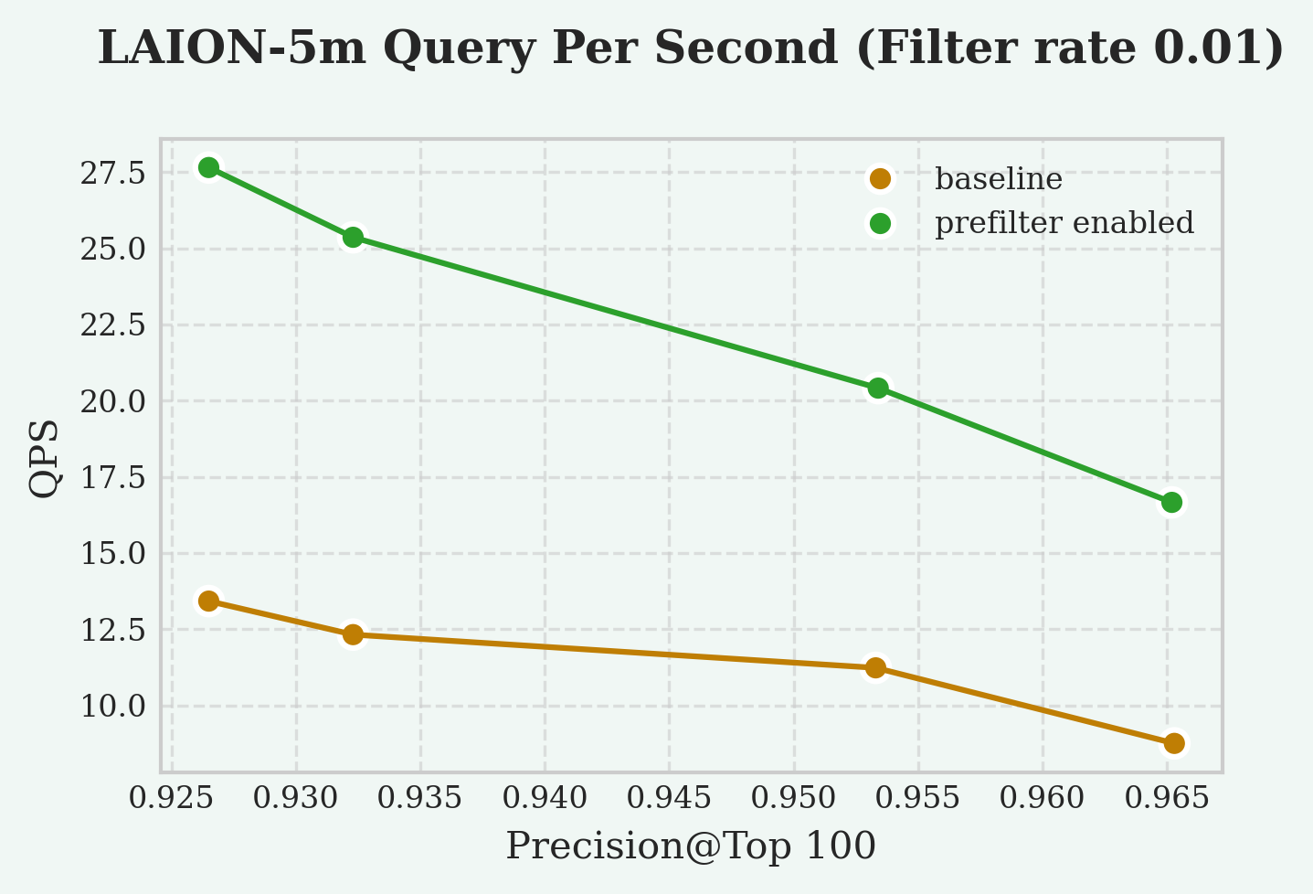
Reference
This feature is not supported by vchordg.
Search Parameters (vchordrq)
vchordrq
vchordrq.prefilter
since v0.4.0
- Description: The
vchordrq.prefilterGUC parameter enables condition evaluation before distance computation. For example, in the querySELECT * FROM items WHERE id % 2 = 0 ORDER BY embedding <-> '[3,1,2]' LIMIT 5, the index normally computes all usefulembedding <-> '[3,1,2]'distances first and then pass the rows to PostgreSQL, which filters out rows whereid % 2 != 0. This parameter allows the index to pre-evaluate the condition and discard non-matching rows before computing their distances, improving query efficiency. - Type: boolean
- Default:
false
2.12 - Prefetch
Prefetch dramatically accelerates queries that involve I/O operations. It works by proactively reading buffers into operating system page cache or PostgreSQL’s buffer pool based on the actual needs of the index.
Prefetch helps overlap I/O with computation, as well as I/O with other I/O operations, significantly reducing the time spent waiting for buffers during query execution, thereby improving overall query performance.
This feature is enabled by default. Any query can benefit from prefetching with VectorChord 0.4.0 and later versions.
Prior to version 0.4.0, VectorChord used PostgreSQL’s synchronous I/O interface. Since then, VectorChord utilizes asynchronous I/O interface on newer versions of PostgreSQL. The I/O interface used by VectorChord can be controlled via GUC parameters.
In the GUC parameters, the synchronous I/O interface is referred to as read_buffer, the asynchronous I/O interface as read_stream, and VectorChord’s simulated asynchronous interface as prefetch_buffer.
For indexes much smaller than the memory, there is almost no difference among the three prefetch modes. read_stream accelerates all disk-based indexes; however, it is only available on PostgreSQL 17 and 18. To address this, VectorChord provides a simulated asynchronous I/O interface called prefetch_buffer, which is available on all PostgreSQL versions as a fallback for older versions. prefetch_buffer is less effective than read_stream.
| Prefetch Mode | Description | Supported PostgreSQL Versions |
|---|---|---|
read_stream |
Asynchronous I/O interface in PostgreSQL | PostgreSQL 17, 18 |
prefetch_buffer |
VectorChord’s simulated asynchronous I/O interface used as fallback on older PostgreSQL versions | PostgreSQL 13, 14, 15, 16, 17, 18 |
read_buffer |
Synchronous I/O interface in PostgreSQL | PostgreSQL 13, 14, 15, 16, 17, 18 |
To fully leverage this feature with read_stream, you need to enable asynchronous I/O on PostgreSQL 18. See also PostgreSQL Tuning.
Reference
Search Parameters (vchordrq)
vchordrq
vchordrq.io_search
since v0.4.0
- Description: This GUC parameter controls the I/O prefetching strategy for reading bit vectors in vector search, which can impact search performance on disk-based vectors.
- Type: string
- Domain: Depends on PostgreSQL version
- PostgreSQL 13, 14, 15, 16:
{"read_buffer", "prefetch_buffer"} - PostgreSQL 17, 18:
{"read_buffer", "prefetch_buffer", "read_stream"}
- PostgreSQL 13, 14, 15, 16:
- Default: Depends on PostgreSQL version
- PostgreSQL 13, 14, 15, 16:
prefetch_buffer - PostgreSQL 17, 18:
read_stream
- PostgreSQL 13, 14, 15, 16:
- Note:
read_bufferindicates a preference forReadBuffer.prefetch_bufferindicates a preference for bothPrefetchBufferandReadBuffer.read_streamindicates a preference forread_stream.
vchordrq.io_rerank
since v0.4.0
- Description: This GUC parameter controls the I/O prefetching strategy for reading full precision vectors in vector search, which can significantly impact search performance on disk-based vectors.
- Type: string
- Domain: Depends on PostgreSQL version
- PostgreSQL 13, 14, 15, 16:
{"read_buffer", "prefetch_buffer"} - PostgreSQL 17, 18:
{"read_buffer", "prefetch_buffer", "read_stream"}
- PostgreSQL 13, 14, 15, 16:
- Default: Depends on PostgreSQL version
- PostgreSQL 13, 14, 15, 16:
prefetch_buffer - PostgreSQL 17, 18:
read_stream
- PostgreSQL 13, 14, 15, 16:
- Note:
read_bufferindicates a preference forReadBuffer.prefetch_bufferindicates a preference for bothPrefetchBufferandReadBuffer.read_streamindicates a preference forread_stream.
Search Parameters (vchordg)
vchordg
vchordg.io_search
since v0.5.0
- Description: This GUC parameter controls the I/O prefetching strategy for reading bit vectors in vector search, which can impact search performance on disk-based vectors.
- Type: string
- Domain: Depends on PostgreSQL version
- PostgreSQL 13, 14, 15, 16:
{"read_buffer", "prefetch_buffer"} - PostgreSQL 17, 18:
{"read_buffer", "prefetch_buffer", "read_stream"}
- PostgreSQL 13, 14, 15, 16:
- Default: Depends on PostgreSQL version
- PostgreSQL 13, 14, 15, 16:
prefetch_buffer - PostgreSQL 17, 18:
read_stream
- PostgreSQL 13, 14, 15, 16:
- Note:
read_bufferindicates a preference forReadBuffer.prefetch_bufferindicates a preference for bothPrefetchBufferandReadBuffer.read_streamindicates a preference forread_stream.
vchordg.io_rerank
since v0.5.0
- Description: This GUC parameter controls the I/O prefetching strategy for reading full precision vectors in vector search, which can significantly impact search performance on disk-based vectors.
- Type: string
- Domain: Depends on PostgreSQL version
- PostgreSQL 13, 14, 15, 16:
{"read_buffer", "prefetch_buffer"} - PostgreSQL 17, 18:
{"read_buffer", "prefetch_buffer", "read_stream"}
- PostgreSQL 13, 14, 15, 16:
- Default: Depends on PostgreSQL version
- PostgreSQL 13, 14, 15, 16:
prefetch_buffer - PostgreSQL 17, 18:
read_stream
- PostgreSQL 13, 14, 15, 16:
- Note:
read_bufferindicates a preference forReadBuffer.prefetch_bufferindicates a preference for bothPrefetchBufferandReadBuffer.read_streamindicates a preference forread_stream.
2.13 - Rerank in Table
PostgreSQL indexes store row identifiers and the values of the indexed columns. Typically, indexed columns have simple data types, for example, integers or strings with short length limits.
However, if the indexed column is of a vector type, both the table and the index store vectors, which means you pay twice the storage cost for the vectors. If you would like to reduce this cost, you can enable rerank_in_table when building the index. The index will then use a tricky approach where it does not store the vectors itself but reads them from the table when needed.
Enabling this option results in degraded query performance and prefetch does not work when rerank_in_table is enabled.
It’s a trade-off of time for space, which is generally not recommended, so it’s intended only to address the specific issue of excessively high storage usage.
Reference
This feature is not supported by vchordg.
Indexing Options (vchordrq)
vchordrq
rerank_in_table
since v0.2.1
- Description: This option determines whether the vectors are fetched from the table. If so, the index will require less storage, but the query latency will increase significantly. It should only be enabled when disk space is extremely limited.
- Type: boolean
- Default:
false - Example:
rerank_in_table = falsemeans that vectors are stored in both the index and the table, and fetched from the index in search.rerank_in_table = truemeans that vectors are stored in the table only, and fetched from the table in search.
2.14 - Partitioning Tuning
For large tables, the partitioning phase dominates both build time and memory consumption.
Time complexity of partitioning is , and the memory consumption in bytes can be approximated by ,
where:
- is the vector dimension, or
build.internal.kmeans_dimensionif set. - is
build.internal.sampling_factor. - is
build.internal.lists[-1]. - is
build.internal.build_threads. - is
build.internal.kmeans_iterations.
This page introduces some tuning techniques to improve build time and memory consumption.
Hierarchical K-means
Hierarchical K-means is an algorithm that is faster than Lloyd’s algorithm. When applied this algorithm, the asymptotic time complexity is reduced to . As a trade-off, it has a slight negative impact on search performance and recall.
Usage:
Reduce Sampling Factor
Reducing sampling factor improves build time and memory consumption linearly. As a trade-off, it has a moderate negative impact on search performance and recall.
Usage:
Dimensionality reduction
Dimensionality reduction uses the fast Johnson–Lindenstrauss transform, reducing the dimensionality of the vectors involved in clustering to below their original dimension, thereby improving build time and memory consumption linearly. As a trade-off, it has a slight negative impact on search performance and recall.
Usage:
Reference settings
LAION 100M
Dataset:
- Source: https://sisap-challenges.github.io/2024/datasets/
- Metric: Inner Product
- Dimension: 768
- Number of vectors: 100,000,000
- Number of test vectors: 1,000
Test machine (AWS EC2 i7i.4xlarge):
- CPU: Intel Xeon Platinum 8559C
- Number of vCPUs: 16
- Memory: 128 GiB
- Storage: 3750 GiB NVMe SSD
Result:
- Total Build Time: 18 minutes
- Peak Memory: 6 GiB
- Test Case 1
- Parameters
vchordrq.probes = '40,140'vchordrq.epsilon = 1.4
- QPS @ Top10: 120
- Recall @ Top10: 0.949
- Parameters
DEEP 1B
Dataset:
- Source: https://big-ann-benchmarks.com/neurips21.html
- Metric: Euclidean
- Dimension: 96
- Number of vectors: 1,000,000,000
- Number of test vectors: 10,000
Test machine (AWS EC2 i7ie.6xlarge):
- CPU: Intel Xeon Platinum 8559C
- Number of vCPUs: 24
- Memory: 192 GiB
- Storage: 7500 GiB NVMe SSD
Result:
- Total Build Time: 107 minutes
- Peak Memory: 64 GiB
- Test Case 1
- Parameters
vchordrq.probes = '40,250'
- QPS @ Top10: 68
- Recall @ Top10: 0.951
- Parameters
2.15 - External Build
In addition to using the methods in Partitioning Tuning to achieve shorter build time and lower memory consumption at the cost of QPS and recall, you can also choose to run the partitioning phase offline on other machines or on GPUs. This feature is not supported by vchordg, since it does not have a partitioning phase.
Assume the table is t and the column to be indexed is val.
Specifically, you need to sample the column for which the index will be built.
Based on these samples, you can partition the vector space into Voronoi cells. After that, you will create a table and insert your partitions.
The index can be created using the following syntax.
Format
The table that stores the partition information must strictly follow the following schema:
- The first column must be
id. Its type isinteger. It must not be null. It must be unique. - The second column must be
parent. Its type isinteger. It could not be null. - The third column must be
vector. Its type isvector. It must not be null.halfvecor other types are not supported yet.
Logically, this forms a tree. The distance from the root to each leaf must be the same.
If any of the above properties are not satisfied, an error will be reported.
Partitioning
To get started, here is a minimal code example for performing partitioning using faiss.
This computes the generators of all Voronoi cells across different levels. The parent-child relationships in the tree are determined by computing the shortest distances, but the details are omitted here. Any algorithm capable of generating multi-level Voronoi cells can be used, such as spherical K-means, balanced K-means or GPU K-means.
3 - Use Cases
| Title | Description | Link | Code |
|---|---|---|---|
| Hybrid search with Postgres Native BM25 and VectorChord | This article explores how to implement Hybrid Search in Postgres using VectorChord-bm25 for keyword-based retrieval and VectorChord for semantic search. | Hybrid Search | Github Repo |
| Supercharge vector search with ColBERT rerank in PostgreSQL | This blog will demonstrate using the PostgreSQL extension VectorChord and pgvector with ColBERT rerank. | ColBERT Rerank | Github Repo |
| Beyond Text: Unlock OCR-Free RAG in PostgreSQL with Modal & VectorChord | This post is your guide to building exactly that: an OCR-free RAG system directly within your familiar PostgreSQL database. We’ll leverage the power of the ColQwen2 Vision Language Model, the efficiency of VectorChord for multi-vector search in Postgres, and the scalability of Modal for GPU-powered embedding generation. | OCR-Free RAG | Github Repo |
3.1 - Hybrid search with Postgres Native BM25 and VectorChord
In the era of RAG (Retrieval-Augmented Generation), efficiently retrieving relevant data from vast datasets is crucial for businesses and developers. Traditional keyword-based retrieval methods, such as those utilizing BM25 as a scoring mechanism, excel in ranking documents based on term frequency and exact keyword matches. This makes them highly effective for structured queries and keyword-heavy content. However, they struggle with understanding synonyms, contextual nuances, and semantic intent. Conversely, vector-based retrieval captures deep semantic meaning, enabling better generalization across varied queries but sometimes sacrificing precision in exact keyword matches. Hybrid Search bridges this gap by combining BM25’s precision with vector search’s contextual understanding, delivering faster, more accurate, and semantically aware results.
This article explores how to implement Hybrid Search in Postgres using VectorChord-bm25 for keyword-based retrieval and VectorChord for semantic search. By leveraging VectorChord-bm25’s BM25 ranking with the Block-WeakAnd algorithm and VectorChord’s advanced vector similarity capabilities, you can build a robust search system that seamlessly integrates keyword precision with semantic understanding. Whether you’re building a recommendation engine, a document retrieval system, or an enterprise search solution, this guide will walk you through the steps to unlock the full potential of hybrid search.
All related benchmark codes can be found here.
Hybrid Search Explained
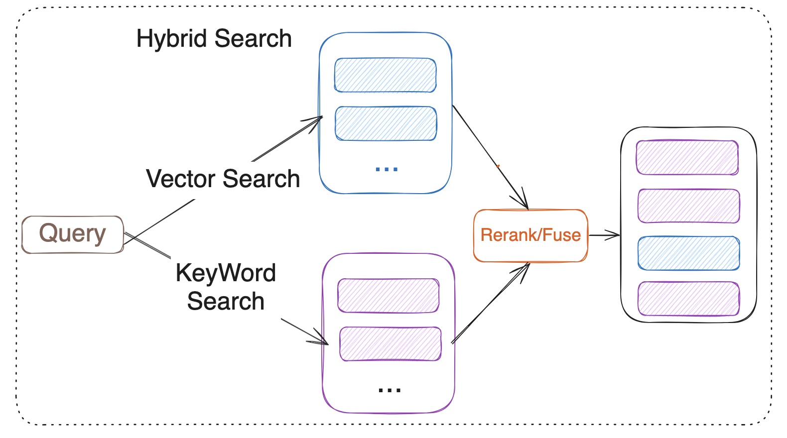
Hybrid Search merges the results from vector search and keyword search. Vector search is based on the semantic similarity between the query and the documents, while keyword search relies on the BM25 ranking algorithm. However, it is important to note that BM25 itself is only responsible for scoring documents, while the broader keyword search process also includes steps such as tokenization, indexing, and query parsing. Hybrid Search utilizes reranker or fuses the results from both methods. Fuses include RRF (Reciprocal Rank Fusion) or weighted scoring for multiple recall strategies. Model-based rerank includes cross encoder models like bge-reranker-v2-m3 and multi-vector representation model ColBERT.
What is the VectorChord?
You may be familiar with pgvector, an open-source vector similarity search extension for Postgres. However, scalable or performance-critical scenarios may require a more advanced vector search solution. VectorChord is an excellent choice.
Check out the blog post “VectorChord: Store 400k Vectors for $1 in PostgreSQL” to learn more about its motivation and design.
What is VectorChord-BM25
VectorChord-BM25 is a PostgreSQL extension for keyword search. It not only implements BM25 ranking but also includes a tokenizer and a Block-WeakAnd index to improve speed.
What is BM25?
BM25 (Best Matching 25) is a probabilistic ranking function used in information retrieval to assess how well a document matches a query. It calculates relevance scores based on term frequency (TF) and inverse document frequency (IDF), while also applying document length normalization. The formula ensures that terms appearing frequently within a document (TF) and those rare across the corpus (IDF) are appropriately weighted, improving search accuracy and relevance. IDF measures how often a word appears across the document collection. The fewer the occurrences, the higher its value. TF represents the frequency of a specific word from the query appearing in the given document. A higher TF indicates a stronger relevance between the query and the document.
Why a Postgres native BM25 Ranking implementation is needed?
In our previous blog post, VectorChord-BM25: Revolutionizing PostgreSQL Search with BM25 Ranking — 3x Faster Than Elasticsearch, my colleague Allen has already provided a detailed and sufficient explanation, which can be referred to.
Tutorial: Use VectorChord-BM25 and VectorChord implement Hybrid Search
In this tutorial, we will guide you through the steps to implement Hybrid Search using VectorChord-BM25 and VectorChord in PostgreSQL. We will cover the following topics:
-
Semantic Search with VectorChord
-
Keyword Search with VectorChord-BM25
-
Rerank
Prerequisites
- Postgres with VectorChord-BM25 and VectorChord
If you want to reproduce the tutorial quickly, you can use the tensorchord/vchord-suite image to run multiple extensions which are provided by TensorChord.
You can run the following command to build and start the Postgres with VectorChord-BM25 and VectorChord.
- Prepare the Embedding Model and Data
For embedding, we can use a pre-trained embedding model like BGE-M3 to generate embeddings for the documents. BGE-M3 is a high-quality embedding model known for its versatility in multi-functionality, multi-linguality, and multi-granularity.
For validation, we use the BEIR dataset, a heterogeneous benchmark for information retrieval. It is easy to use and allows you to evaluate your models across 15+ diverse IR datasets.
First, you need to load your data into PostgreSQL. Then you can use the following SQL query to generate embeddings for the documents.
For embedding:
The data process and embedding generation code can be found here.
Semantic Search with VectorChord
For semantic search, we utilize the RaBitQ algorithm, which is highly optimized in the VectorChord PostgreSQL extension. RaBitQ is a quantization algorithm for high-dimensional spaces, designed to improve the storage and retrieval efficiency of high-dimensional data, such as embedded vectors.
It achieves this by mapping high-dimensional vectors to a low-dimensional discrete space while preserving the similarity information of the original vectors. This process reduces storage requirements and computational costs while maintaining high retrieval accuracy.
If you find that building the index on your own dataset is too slow, you can utilize external build to accelerate the process. For more details, please refer to our previous blog: Benefits and Steps of External Centroids Building in VectorChord.
Once the index is built, you can use the following SQL query to search for similar documents:
Key-Word Search with VectorChord-BM25
For keyword search, we need to use a tokenizer to convert the text into a BM25 vector, which is similar to a sparse vector that stores the vocabulary ID and frequency.
Let me explain this operation in detail. The tokenize function is used to tokenize the text with the specified tokenizer. In this case, we used the Unicode tokenizer. The output of the tokenize function is a BM25 vector, which is a sparse vector that stores the vocabulary ID and frequency of each word in the text. For example, 1035:7 means the word with vocabulary ID 1035 appears 7 times in the text.
After creating the index, you can calculate the BM25 score between the query and the vectors. Note that the BM25 score is negative, meaning that the higher the score, the more relevant the document is. We intentionally make it negative so that you can use the default ORDER BY to retrieve the most relevant documents first.
Rerank/Fuse
Once you obtain the results from both semantic search and keyword search, you can use a fuse or rerank process to merge the results.
- Fuse (Reciprocal Rank Fusion (RRF))
The advantage of RRF lies in its independence from specific score units; it is based on ranking for fusion, making it suitable for sorting systems with different scoring criteria.
Among them:
-
dis the document. -
nis the number of ranking systems. -
rankis the ranking in the sorting system. -
kis the adjustment parameter, the value is usually 60 (empirical value), used to control the impact of ranking on scores.
- Cross-Encoder model Rerank
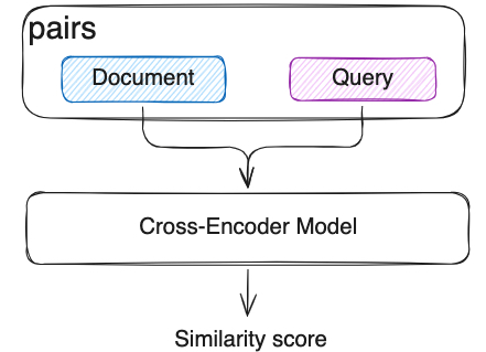
In semantic search, we already use Bi-Encoder vectorized the documents and queries separately. But this independent encoding leads to a lack of interaction between the query and the document. Cross-Encoder model will input the query and document as a whole into the model, the model will see the content of both at the same time, capturing the fine-grained semantic relationship between them through the Transformer layer. Compared with RRF, Cross-Encoder model can capture the fine-grained semantic relationship between the query and the document, and it can be more accurate but slower.
Evaluation
We have tested the NDCG@10 with those methods on several BEIR datasets. Here are the top10 results:
| Dataset | Semantic Search | BM25 | Cross-Encoder Rerank | RRF |
|---|---|---|---|---|
| FiQA-2018 | 0.40343 | 0.25301 | 0.42706 | 0.37632 |
| Quora | 0.88433 | 0.78687 | 0.89069 | 0.87014 |
| SCIDOCS | 0.16055 | 0.15584 | 0.17942 | 0.17299 |
| SciFact | 0.57631 | 0.68495 | 0.74635 | 0.67855 |
The table above demonstrates several conclusions:
-
Compared to BM25 and semantic search, the cross-encoder model rerank can significantly improve search performance across different datasets.
-
On some datasets, RRF may lead the performance decrease. Please conduct verification tests before deciding whether to use RRF. If effective, choosing RRF will be a very economical choice, as it is much, much faster than reranking with the cross-encoder model, and almost no resource consumption.
All related benchmark codes can be found here. If you have any questions, please feel free to contact us on Discord or email us at rh@vonng.com.
Future Work
The results highlight the great potential of the hybrid search method. In the future, we will focus on the following aspects to advance RAG:
- Improve the reranking method: Explore the other model-based rerank, such as ColBERT or ColPali, to enhance reranking performance.
- Integrate graph search: Investigate the use of the Apache AGE extension for graph search and integrate it with the hybrid search method to further improve search performance.
References
- https://github.com/pgsty/vchord
- https://github.com/pgsty/vchord_bm25
- https://techcommunity.microsoft.com/blog/adforpostgresql/introducing-the-graphrag-solution-for-azure-database-for-postgresql/4299871
- https://www.pinecone.io/learn/hybrid-search-intro/
- https://www.pinecone.io/learn/series/rag/rerankers/
- https://blog.vespa.ai/improving-zero-shot-ranking-with-vespa-part-two/
3.2 - Supercharge vector search with ColBERT rerank in PostgreSQL
Traditional vector search methods typically employ sentence embeddings to locate similar content. However, generating sentence embeddings through pooling token embeddings can potentially sacrifice fine-grained details present at the token level. ColBERT overcomes this by representing text as token-level multi-vectors rather than a single, aggregated vector. This approach, leveraging contextual late interaction at the token level, allows ColBERT to retain more nuanced information and improve search accuracy compared to methods relying solely on sentence embeddings.
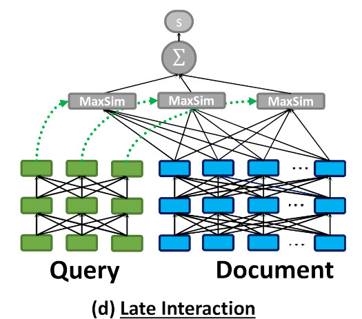
As illustrated in the above image, ColBERT encodes each document/query into a list of token vectors and computes the MaxSim during the query time.
Token-level late interaction requires more computing power and storage. This makes using ColBERT search in large datasets challenging, especially when low latency is important.
One possible solution is to combine sentence-level vector search with token-level late interaction rerank, which leverages the efficiency of approximate vector search and the high quality of multi-vector similarity search.
The multi-vector approach is not limited to pure text retrieval tasks; it can also be used in visual document understanding. For multimodal retrieval models, state-of-the-art models like ColPali and ColQwen directly encode document images into multi-vectors and demonstrate stronger performance compared to OCR-to-text approaches.
This blog will demonstrate using the PostgreSQL extension VectorChord and pgvector with ColBERT rerank.
Tutorial
Assume we already have the documents, let’s create a table to store all of them:
Here we created a table with sentence-level embedding and token-level embeddings.
There are numerous embedding APIs and open-source models. You can choose the one that fits your use case.
For token-level embedding:
ColBERT model produces 128-dim vectors by default.
To insert the data:
For the vector search part, we can use VectorChord to build a high-performance RaBitQ index:
To speed up the indexing building process, we can utilize the external centroids build. Check “Benefits and Steps of External Centroids Building in VectorChord” for more details.
Now, we can query the PostgreSQL:
To support MaxSim rerank, we’ll need to create a function:
Now, we can rerank the documents retrieved by vector search:
Evaluation
We have tested this method on several BEIR datasets. Here are the results:
| Dataset | Search NDCG@10 | Rerank NDCG@10 |
|---|---|---|
| fiqa | 0.23211 | 0.3033 |
| quora | 0.31599 | 0.3934 |
This shows that ColBERT reranking can significantly enhance the results of vector searches.
All the related benchmark codes can be found here.
Future work
Vector search and full-text search with ColBERT rerank can further improve performance. We’re also working on the PostgreSQL BM25 extensions. Stay tuned.
References
3.3 - Beyond Text: Unlock OCR-Free RAG in PostgreSQL with Modal & VectorChord
Building effective Retrieval-Augmented Generation (RAG) systems for documents often feels like wrestling with messy, complex pipelines. Especially when dealing with PDFs or scanned images, traditional methods rely heavily on Optical Character Recognition (OCR) and layout analysis. These steps can be slow, error-prone, and often lose crucial visual context like tables, figures, and formatting. But what if you could query documents based on how they look, not just the extracted text?
This post is your guide to building exactly that: an OCR-free RAG system directly within your familiar PostgreSQL database. We’ll leverage the power of the ColQwen2 Vision Language Model, the efficiency of VectorChord for multi-vector search in Postgres, and the scalability of Modal for GPU-powered embedding generation. Get ready to simplify your RAG stack and potentially boost your retrieval accuracy, all without complex pre-processing.
We’ll cover:
-
What ColQwen2 is and why it’s a game-changer.
-
How VectorChord makes advanced vector search possible in Postgres.
-
A step-by-step tutorial to build and evaluate the system.
What is ColQwen2? The Power of Visual Understanding
To grasp ColQwen2, let’s first look at its foundation: ColPali. As introduced in the paper “ColPali: Efficient Document Retrieval with Vision Language Models”, ColPali represents a novel approach using Vision Language Models (VLMs). Instead of relying on imperfect OCR, it directly indexes documents using their rich visual features – text, images, tables, layout, everything the eye can see.
Think about the limitations of traditional OCR: complex layouts get mangled, tables become gibberish, and images are often ignored entirely. It’s like trying to understand a book by only reading a flawed transcript. ColPali avoids this by using a powerful VLM (originally PaliGemma) to create embeddings that capture the document’s holistic visual nature. Two key concepts make it shine:
-
Contextualized Vision Embeddings: Generating rich embeddings directly from the document image using a VLM.
-
Late Interaction: This clever technique allows the query’s textual meaning to directly interact with the document’s detailed visual features at search time. It’s not just matching text summaries; it’s comparing the query concept against the visual evidence within the document page.

The ColPali architecture (Image from the ColPali paper)
ColQwen2 builds upon this powerful ColPali architecture but swaps the underlying VLM for the more recent Qwen2-VL-2B. It generates ColBERT-style multi-vector representations, capturing fine-grained details from both text and images. As seen on the vidore-leaderboard, ColQwen2 delivers impressive performance with practical model size.
How Does VectorChord Enable ColQwen2 in Postgres?
This is where VectorChord becomes the crucial piece of the puzzle, bringing this cutting-edge VLM capability into your PostgreSQL database. ColQwen2 (and ColPali) relies heavily on those multi-vector representations and the Late Interaction mechanism, specifically requiring an efficient MaxSim (Maximum Similarity) operation.
Calculating MaxSim – finding the highest similarity score between any vector in the query set and any vector in the document set – can be computationally brutal, especially across millions of document vectors. VectorChord tackles this head-on:
-
Native Multi-Vector Support: It’s designed from the ground up to handle multi-vector data efficiently within Postgres.
-
Optimized MaxSim: Drawing inspiration from the WARP paper, VectorChord uses techniques like dynamic similarity imputation to dramatically speed up MaxSim calculations, making large-scale visual document retrieval feasible.
-
Hybrid Search Ready: Beyond multi-vector, it also supports dense, sparse, and hybrid search (check out our previous post!).
-
Scalable & Disk-Friendly: Designed for performance without demanding excessive resources.
In short, VectorChord transforms PostgreSQL into a powerhouse capable of handling the advanced vector search techniques required by models like ColQwen2 or ColPali.
Tutorial: Building Your OCR-Free RAG System
Alright, theory’s great, but let’s roll up our sleeves and build this thing! We’ll walk through setting up the environment, processing data using Modal for scalable embedding generation, indexing into VectorChord within Postgres, and finally, evaluating our shiny new OCR-free RAG system.
Prerequisites
Before we start, ensure you have:
-
A PostgreSQL instance (Docker recommended) with the VectorChord extension installed OR a VectorChord Cloud cluster.
-
A Modal account (free tier available). Modal’s fast GPU provisioning and scaling are perfect for the embedding generation step. To efficiently process a large volume of documents using the ColQwen2 model, it’s crucial to leverage Modal’s rapid startup and GPU expansion features. This approach will significantly reduce the time required for local processing.
If you want to reproduce the tutorial quickly, you can use the tensorchord/vchord-suite image to run multiple extensions that TensorChord provides.
You can run the following command to build and start Postgres with VectorChord-BM25 and VectorChord.
Set up Modal:
Step 1: Load the Data (Using Modal Volumes)
We’ll use the ViDoRe Benchmark dataset. To handle this data efficiently across potentially distributed Modal functions, we’ll download it to a Modal Volume. Volumes provide persistent, shared storage ideal for this ‘download once, process many times’ scenario.
Modal offers a straightforward Python API for interacting with its platform. With modal.Image, you can set the base image for the Modal App, and the function decorator helps define the function to be executed within the Modal application. To download the dataset to the Modal Volume, execute the following command. Modal will then automatically build the Docker image and promptly launch the container to run your function.
Run the download function:
Modal handles building the environment and running the script in the cloud.
Step 2: Process Data & Generate Embeddings (With Modal & ColQwen2)
This is the heavy lifting: converting document images into ColQwen2 multi-vector embeddings. Doing this locally for many documents would be slow. Modal shines here:
-
Easy GPU Access & Autoscaling: Launch a ColQwen2 model service on Modal and use it to generate the image embeddings and query embeddings for the dataset. The decision to implement an HTTP service instead of using the SDK directly was made to ensure seamless auto-scaling during large-scale embedding operations. If you want to deploy the embedding service as a persistent web endpoint, you can directly change
modal.clstomodal.web_serverfor ColPaliServer and runningmodal deploy. -
Recovery: We checkpoint progress to a separate Modal Volume, allowing us to resume embedding generation if interrupted.
Generate the embeddings:
Step 3: Create Index in VectorChord (Using Vechord SDK)
With embeddings generated and saved in a Modal Volume, we first need to bring them local.
Now, we’ll use the vechord SDK to load these embeddings into our PostgreSQL database and create the necessary multi-vector index. vechord provides a Pythonic, ORM-like way to interact with VectorChord in Postgres.
%[https://github.com/tensorchord/vechord]
Run the indexer script, vechord handles table creation, index creation, and data insertion.
Step 4: Evaluation - Does it Work?
The final step is crucial: evaluating retrieval performance. Does this OCR-free system deliver accurate results, and can it be fast? We’ll use vechord to run queries against our indexed data and look at NDCG@10 and Recall@10. We’ll also test the impact of VectorChord’s WARP optimization, which accelerates MaxSim calculations. In this tutorial, we will use vidore/arxivqa_test_subsampled dataset for evaluation queries, the data are shown below.
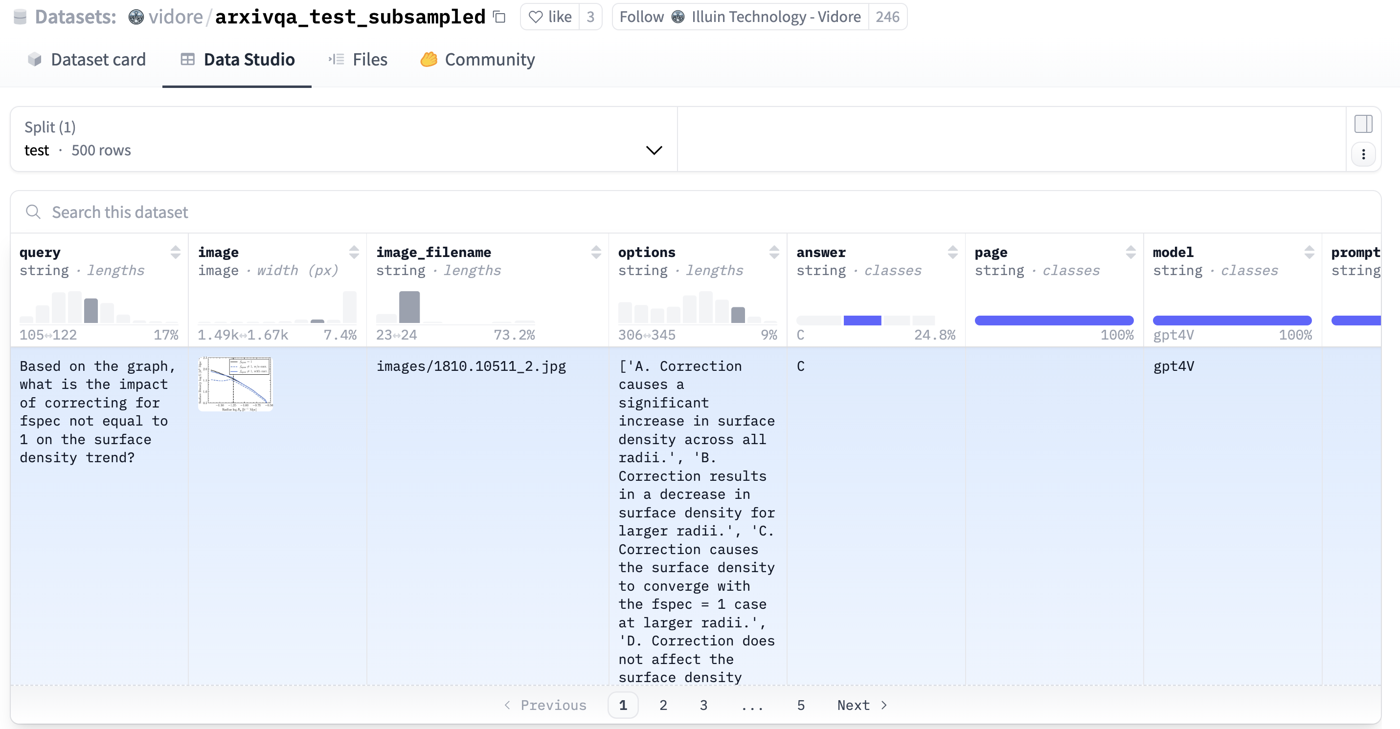
Running the evaluation script yields impressive results:
Analysis:
-
High Baseline Accuracy: First, let’s look at the baseline performance without WARP optimization. The system achieves an excellent NDCG@10 of 0.8615 and Recall@10 of 0.92. This confirms the fundamental effectiveness of ColQwen2 embeddings paired with VectorChord’s precise MaxSim search, delivering state-of-the-art results for visual document retrieval even without speed optimizations.
-
Dramatic WARP Speed Boost: Now, observe the impact of enabling VectorChord’s WARP optimization. The total execution time plummets from a substantial 810 seconds down to just 41 seconds! This represents a massive ~18.7x speedup for the evaluation query set. This clearly demonstrates WARP’s power in dramatically accelerating the computationally intensive MaxSim operations required for late-interaction models like ColQwen2.
-
Minimal Accuracy Trade-off: Impressively, this significant speed gain comes at the cost of only a very minor dip in retrieval accuracy. The NDCG@10 slightly decreases to 0.8353 (a difference of less than 0.3), and Recall@10 reduces minimally to 0.9 (a difference of only 0.02).
Conclusion: Visual RAG Made Simpler in Postgres
In this tutorial, we successfully built a high-performance, OCR-free RAG system by bringing together the visual understanding capabilities of ColQwen2, the scalable multi-vector search of VectorChord within PostgreSQL, and the efficient GPU processing of Modal. We saw how this stack allows us to directly query documents based on their visual content, bypassing the pitfalls of traditional OCR pipelines.
The ability to seamlessly integrate this visual dimension into your RAG system directly within Postgres opens up exciting possibilities for applications dealing with visually rich documents like scientific papers, invoices, product manuals, historical archives, and much more.
Ready to try it yourself?
-
Explore the Code: https://github.com/xieydd/vectorchord-colqwen2
-
Dive Deeper into VectorChord: Check out the VectorChord documentation or try the hassle-free VectorChord Cloud.
-
Experiment: Try different VLMs or datasets.
-
Share Your Thoughts: Let us know your experiences or questions in the comments below!
This approach represents a significant step towards simpler, more robust, and visually-aware document retrieval systems.
References
4 - Benchmarks
4.1 - Price Benchmark
Using VectorChord, you can achieve a QPS of 131 with 0.95 precision on 100 million 768-dimensional vectors for the top 10 queries. This setup costs only $250 monthly and can be hosted on a single machine. If you are interested in the details of our implementation, please refer to our blog VectorChord: Store 400k Vectors for $1 in PostgreSQL.
This means you can store 400k vectors for only $1, allowing you to save significantly: 6x more vectors compared to Pinecone (storage optimized instance) and 26x more than pgvector/pgvecto.rs for the same price.
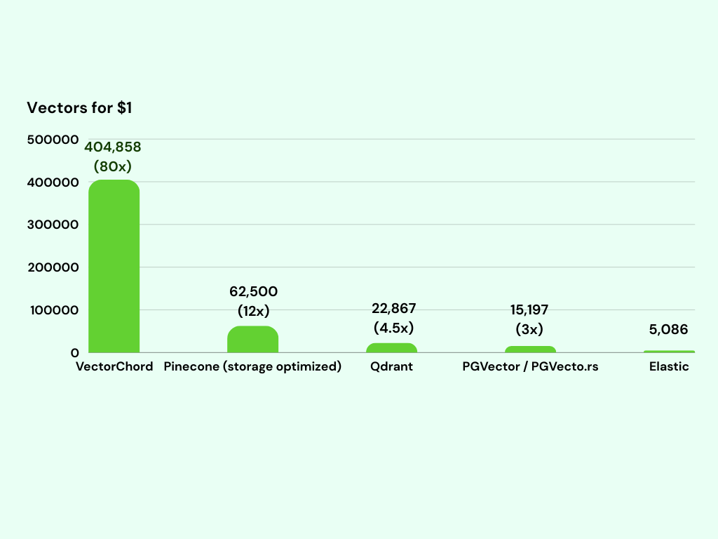
In the monthly cost comparison for storing vectors, based on MyScale benchmark data, the chart highlights how VectorChord emerges as an affordable option, priced at just $247 for storing 100 million vectors. In contrast, Pinecone, despite its optimized storage, costs $1,600 per month, while Qdrant is priced at $4,374. pgvector/pgvecto.rs has a considerably higher cost of $6,580.
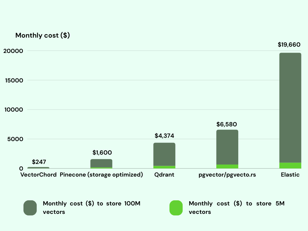
The price benchmark is tested on December 5, 2024. We are ongoingly enhancing performance and optimizing costs. For example, VectorChord 0.2 builds on its predecessor with a 30% smaller index size and 50% faster builds. If you want to know the latest benchmark, please contact us at discord.
4.2 - Performance Benchmarking
Here we present a comprehensive benchmark comparing our implementation of VectorChord with other vector databases, focusing on QPS and scalability. If you are interested in the details of our implementation, please refer to our blog VectorChord: Store 400k Vectors for $1 in PostgreSQL.
QPS
LAION 5M
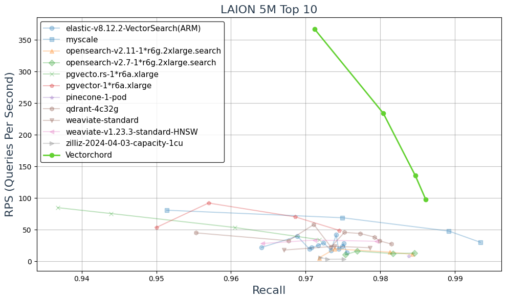
In LAION 5M dataset, VectorChord achieved more than 3x QPS at 0.95 recall compared to different vector databases, including MyScale, pgvector, pinecone, weaviate, qdrant and zilliz(milvus).
LAION 100M on i4i.xlarge
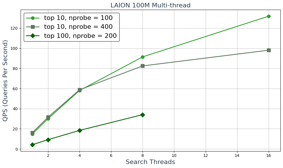
This setup utilizes 4 CPUs and 32 GB of memory, with 937 GB of SSD storage for the 100 million vectors. We achieved a QPS of 16.2 at a recall rate of 0.95 for the top 10 results and 4.3 at 0.95 for the top 100, using a single-threaded query. The results are truly impressive.
Scalability
If you are interested VectorChord scalable capability, you can refer our blog Vector Search at 10,000 QPS in PostgreSQL with VectorChord.
LAION 100M && LAION 5M
| dataset | minimal hardware for 10000+ QPS | number of vcpu | estimate cost per month |
|---|---|---|---|
| LAION-5m | r7i.xlarge × 7 | 4 × 7 = 28 vcpu | $0.2646 × 7 × 720 = $1334 |
| LAION-100m | r7i.16xlarge × 2 | 64 × 2 = 128 vcpu | $4.2336 × 2 × 720 = $6096 |
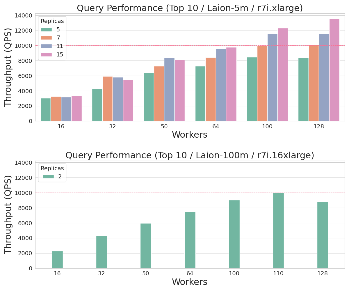
The price benchmark is tested on December 5, 2024. We are ongoingly enhancing performance and optimizing costs. For example, VectorChord 0.2 builds on its predecessor with a 30% smaller index size and 50% faster builds. If you want to know the latest benchmark, please contact us at discord.
4.3 - Benchmark with pgvector
In this section, we compare VectorChord with pgvector, a PostgreSQL extension that provides vector similarity search capabilities. We will focus on four key metrics: QPS (Queries Per Second), Recall@100, Index Building Time, and Insertion Time. If you are interested in the details of our implementation, please refer to our blog Vector Search Over PostgreSQL: A Comparative Analysis of Memory and Disk Solutions.
QPS & Recall
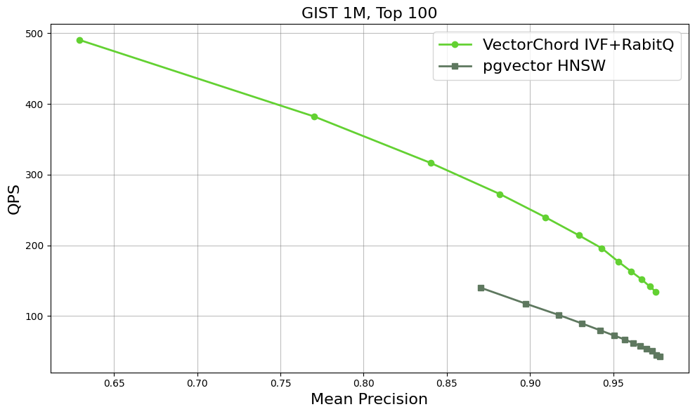
Here are some initial benchmark results for the GIST dataset, which consists of 1 million vectors in 960 dimensions. With equivalent recall, VectorChord’s QPS could be twice that of pgvector. More details will be provided in the Benchmark section.
Index Build Time & Insert Time & Query Completion Time
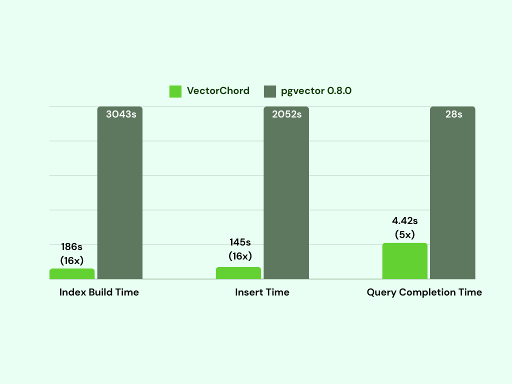
VectorChord takes 186 seconds to build the index by utilizing a separate machine for KMeans clustering, making it 16 times faster than pgvector. Additionally, the insert time is also 14 times faster than that of pgvector. As we know, indexing is the most resource-intensive part of vector databases, requiring significant computation and increasing the demand for CPUs and memory. By utilizing a more capable machine to build the index and then importing it to a smaller machine for querying, it becomes possible to support billions of vectors on a single machine.
4.4 - Benchmark with Elasticsearch
Here we present a comprehensive benchmark comparing our implementation of VectorChord-BM25 with ElasticSearch, focusing on two key metrics: QPS (Queries Per Second) and NDCG@10 (Normalized Discounted Cumulative Gain at rank 10). If you are interested in the details of our implementation, please refer to our blog VectorChord-BM25: Revolutionize PostgreSQL Search with BM25 Ranking — 3x Faster Than ElasticSearch.
RPS
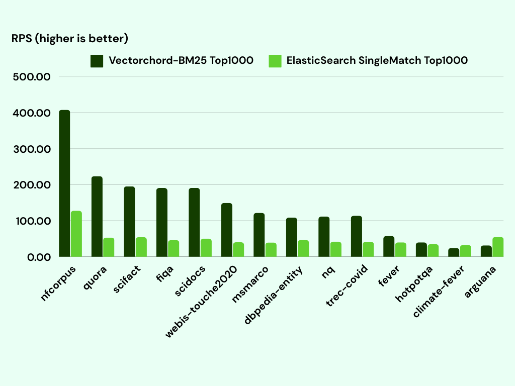
We compare the Top1000 Queries Per Second (QPS)—a metric that measures how many queries a system can process per second while retrieving the top 1000 results for each query—between our implementation and ElasticSearch across various datasets from bm25-benchmarks. On average, our implementation achieves 3 times higher QPS compared to ElasticSearch across the tested datasets, showcasing its efficiency and scalability.
NDCG@10
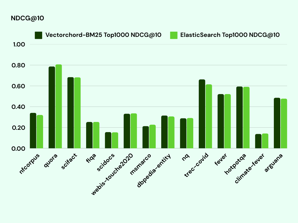
We have dedicated substantial effort to align VectorChord-BM25 with ElasticSearch’s behavior, ensuring a fair and precise comparison. As demonstrated in the table, our implementation achieves NDCG@10 scores that are comparable across most datasets, with certain cases even surpassing ElasticSearch (e.g., trec-covid and scifact).
4.5 - Benchmark with pgvectorscale
In this section, we compare VectorChord with pgvectorscale, a PostgreSQL extension that provides vector similarity search capabilities. We will focus on four key metrics: QPS (Queries Per Second), Recall@10/100, Index Building Time, and Insertion Time. Memory and disk performance will also be discussed. If you are interested in the details of our implementation, please refer to our blog Vector Search Over PostgreSQL: A Comparative Analysis of Memory and Disk Solutions.
QPS & Recall
Memory
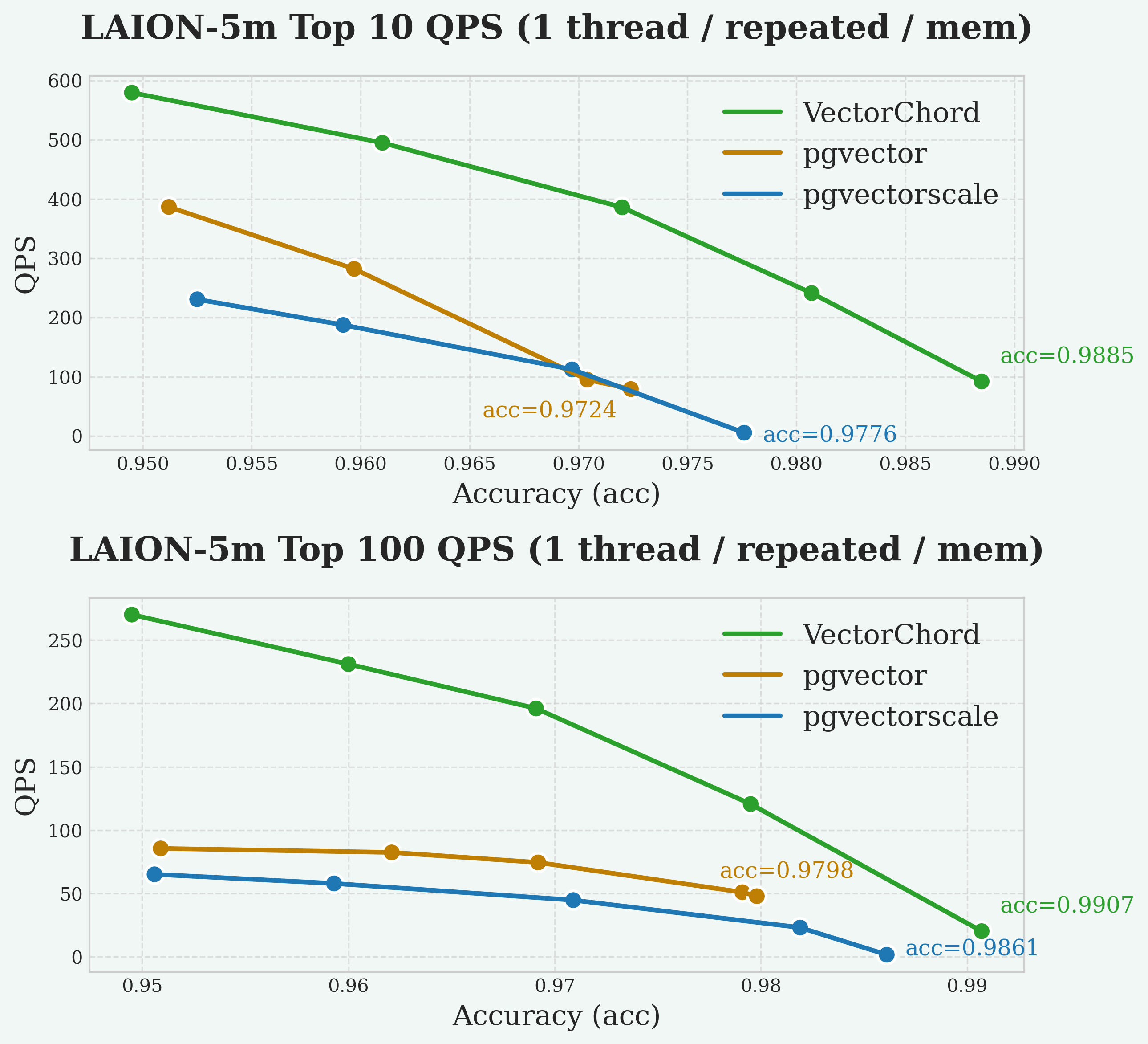
The graphs illustrate the trade-off between query speed (QPS) and search quality (Recall@10/100). Recall@10 measures the percentage of true nearest neighbors found within the top 10 results. In general, higher QPS can be achieved at the cost of lower recall, and vice versa. A better system may achieve higher recall at the same QPS, or higher QPS at the same recall level. Our goal is typically to maximize QPS while maintaining a high recall target (e.g., 95%).
Disk
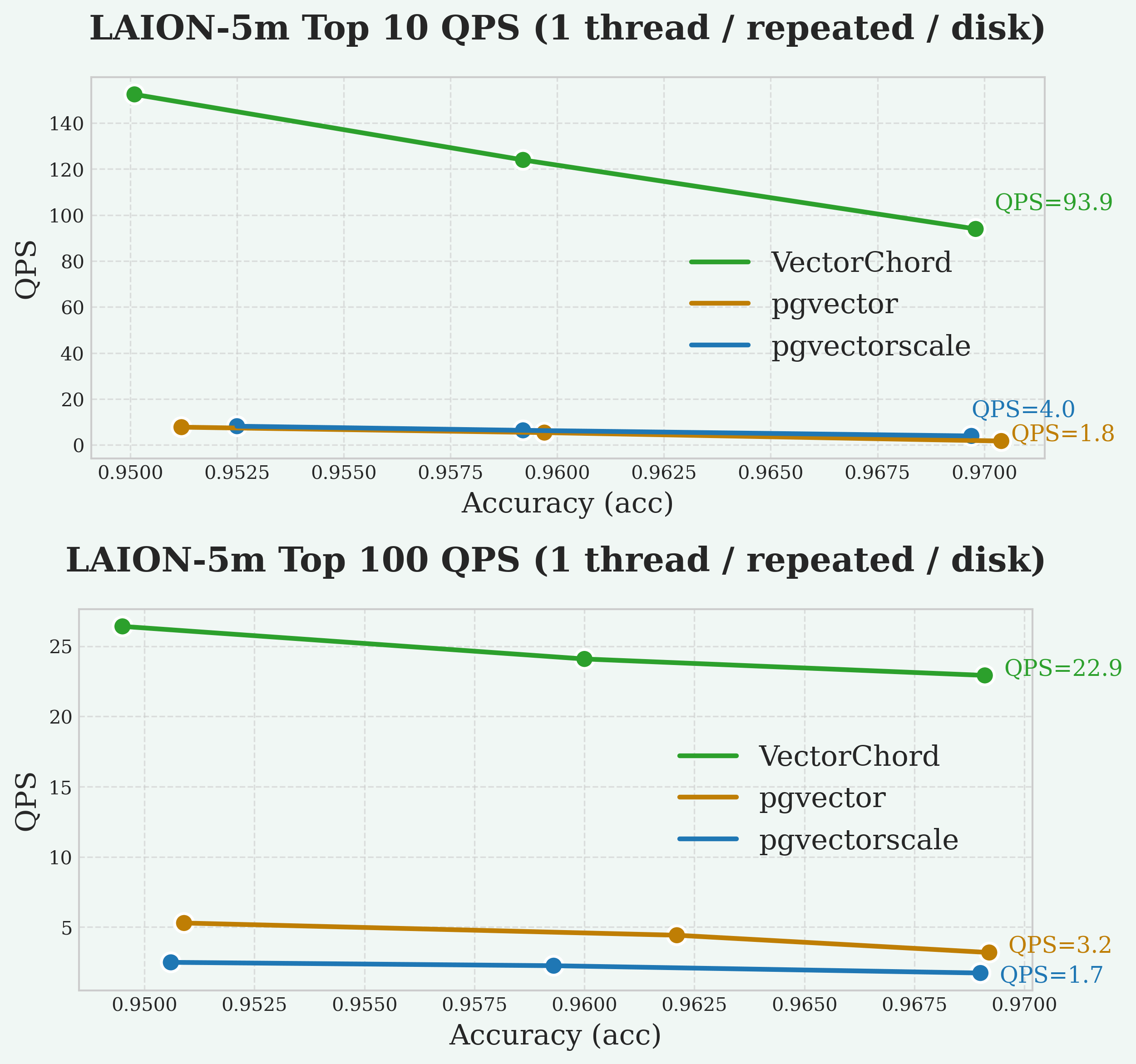
As always, VectorChord consistently achieves higher QPS at high recall levels (e.g., >95% Recall@10) compared to the other extensions, followed by pgvector and pgvectorscale with similar QPS.
Index Building
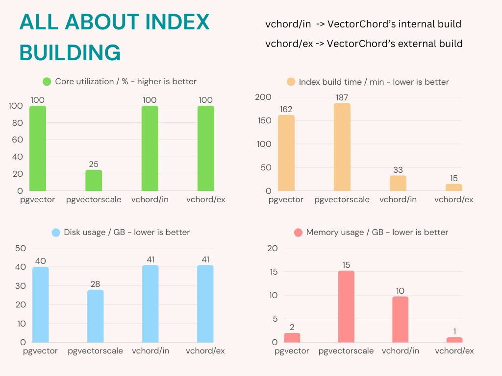
VectorChord maximizes CPU usage, reduces memory consumption, and shortens index-building time compared to pgvectorscale.
Insertion Time
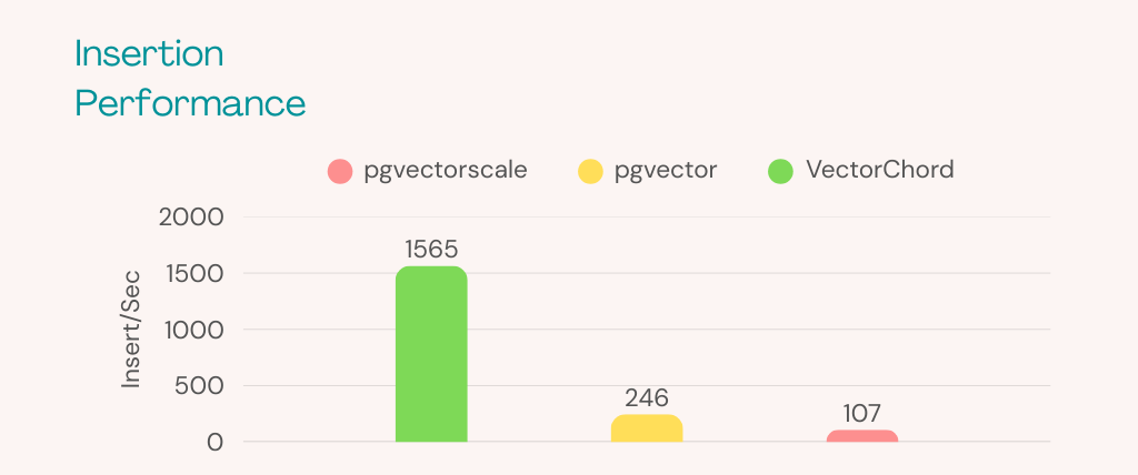
As you can see, VectorChord (1565 Insert/Sec) performs much better than pgvector (246 Insert/Sec) and pgvectorscale (107 Insert/Sec) when inserting data. For most workloads, 100 Insert/Sec is more than enough. However, if you find that a lot of vectors are continuously inserted in your production (for example, 500 Insert/Sec), this could be a problem.
5 - Administration
5.1 - Migration
outline: [2,3]
VectorChord Migration Overview
From PGVecto.rs
Most of VectorChord’s vector types are supported by pgvector.
Therefore, migrating from PGVecto.rs to VectorChord is a simple inversion of migrating from pgvector to PGVecto.rs.
We provide migration image modelzai/pgvectors-vchord for pgvecto.rs to VectorChord and vice versa.
Prerequisites
Let’s suppose that you have a table with vector data, and the extension PGVecto.rs installed. A simple example would be:
In addition, some rows will be inserted into the table, as follows:
In most cases, there will also be one or more vector indexes:
This is a typical scenario when PGVecto.rs is used. If the following requirements are met, the migration can be initiated.
- Please note that your
pgvectorandVectorChordextension is not installed in thevectorsschema. This means that you can installpgvectorandPGVecto.rsat the same time.
Steps to Migration
1. Install VectorChord
Please follow the instructions provided to install VectorChord and ensure that the extension is loaded by PostgreSQL.
This will install vectorchord and pgvector at public schema, if other schema is picked, please substitute public with your schema at the migration command.
The two extensions VectorChord and PGVecto.rs are now installed on PostgreSQL, but inside different schemas.
To validate it, please run \dx in psql. You will see that there are 3 extensions:
vectorsforPGVecto.rsat schema vectorsvectorforpgvectorat schema publicvchordforVectorChordat schema public
2. Check existing indexes
For indexes created at vector columns, please retrieve the definition and record it in a convenient location. This information is necessary for the recovery of the indexes at a later stage.
3. Migrate vector columns
To migrate from a PGVecto.rs vector column, the first step is to cast column datatypes between extensions.
Here provides the conversion path for each vector type of VectorChord:
vector(PGVecto.rs) -> real[] -> vector(pgvector)vecf16 -> vector(PGVecto.rs) -> real[] -> halfvecbvector -> vector(PGVecto.rs) -> text[] -> real[] -> bitsvector -> text -> index++ -> text -> sparsevec
For sparse vector type svector, we need additional helper function to finish the casting, see the appendix.
The migration will be completed in one command and no additional memory is required. However, you need to delete the index on the vector column in advance.
This step will cause some downtime, due to:
- a long
ACCESS EXCLUSIVElock byALTER TABLE ALTER COLUMN
4. Recreate index
The next step is to recreate index on vector columns for PGVecto.rs.
For more information on creating index at VectorChord, see indexing.
5. Clean the environment
You may now safely remove the PGVecto.rs extension if it is no longer required.
Appendix: cast of sparse vector
We have discussed most types, but not the sparse vector. It is a little more complicated than other types. Suppose we have a table with a sparse vector column:
Sparse vectors have a different text representation between PGVecto.rs and pgvector: The index starts from 0 in PGVecto.rs and from 1 in pgvector.
For example, a typical sparse vector [-1, 0, 1, 0, 2] has a text representation of:
{0:-1, 2:1, 4:2}/5inPGVecto.rs{1:-1, 3:1, 5:2}/5inpgvector
So we need a helper function to handle this change by processing the string:
After that, the migration can continue smoothly:
5.2 - Scalability
Background
High queries per second (QPS) vector search is essential for real-time applications such as recommendation engines, image recognition, and natural language processing. These applications demand rapid, efficient searches to deliver immediate results, which is critical for maintaining user engagement and operational effectiveness. By leveraging PostgreSQL for vector search, you not only benefit from its mature, robust relational capabilities and advanced indexing but also avoid the overhead of managing a separate, specialized vector database. This unified approach simplifies integration and reduces system complexity while still meeting the performance needs of modern applications.
Architecture
Using VectorChord on a multi-node cluster is more difficult than on a single machine. As with other services, a reliable distributed vector search usually has the following requirements:
-
Usability: Declarative configuration management
-
Elasticity: Automatic scaling for nodes based on QPS requirements
-
Load Balancing: Requests are handled effectively across different replica instances
-
High Availability: Having multiple copies of the database and automatically recovering from a replica in case of failure
-
Durability: Secure, persistent storage to ensure data integrity and prevent loss in the event of failures
Therefore, we deploy VectorChord services on AWS EKS with OpenTofu and CloudNativePG to manage the infrastructure that provides the above capabilities. Here are some modules to build the example clusters:
-
OpenTofu: Open source alternative of terraform, used for infrastructure as code (IaC) on AWS EKS
-
CloudNativePG: Manage the full lifecycle of a highly available PostgreSQL database cluster with a primary/standby architecture
-
PGBouncer: Lightweight connection pooler for PostgreSQL, provided by module Pooler of CloudNativePG
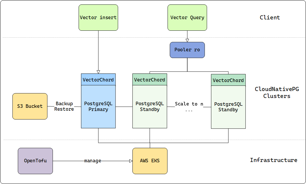
Similar to DiskANN, VectorChord can fully utilize disk resources and still maintain competitive performance when memory is insufficient. Besides, VectorChord can also cache indexes in memory to achieve higher query performance.
For more on the technical details of VectorChord, please see our previous blog.
To reach the QPS limit, we should assume that the memory can fully hold the dataset and select the AWS machine type based on this standard.
In the following table, we provide the appropriate machine which can hold everything in memory for different sizes of datasets:
| dataset | dim / size | machine / memory |
|---|---|---|
| LAION-5m | 768 / 5,000,000 | r7i.xlarge / 32GB |
| LAION-100m | 768 / 100,000,000 | r7i.16xlarge / 512GB |
Results
As outlined in our documentation, VectorChord accepts two key parameters: nprob and epsilon. Here, nprob defines the number of candidate vectors to scan during a query, while epsilon serves as the threshold for determining whether to rerank results. Both parameters play a critical role in influencing both QPS and recall, allowing users to fine-tune the balance between search speed and accuracy.
-
Lower
nprobwill result in higher QPS and lower recall. -
Lower
epsilonwill result in higher but more unstable QPS and lower recall.
If these parameters are fixed, the precision of each experiment will remain consistent. However, the QPS will still vary depending on the CPU and I/O performance of the underlying hardware. To ensure the precision stays above 0.9, we configured the parameters based on earlier experiments conducted with smaller datasets.
| dataset | nprob / epsilon | recall |
|---|---|---|
| LAION-5m | 20 / 1.0 | 0.9324 |
| LAION-100m | 20 / 1.0 | 0.9042 |
We deployed an r7i.4xlarge instance as the client within the same Availability Zone to query the VectorChord clusters. The clusters were tested with multiple workers ranging from 16 to 128, simulating the concurrency levels typically applied to the database in real-world scenarios. This setup allows us to evaluate how VectorChord performs under varying workloads and concurrency conditions.
With 16 vCPUs, r7i.4xlarge can effectively reduce CPU contention from the client side when the concurrency requests reach up to 128.
In line with common pgbouncer practices, we employed two types of instances: a primary instance for data ingestion and multiple replica instances for read-only workloads. Pgbouncer served as the load balancer, efficiently distributing queries across these backend instances. For the benchmark, we directed our query endpoint to the read-only (ro) pooler, while the read-write (rw) primary instance remained idle during the test. This setup ensures optimal resource utilization and scalability for read-heavy workloads.
For the 5 million dataset, we scaled the number of instances from 5 to 15 to achieve 10,000 QPS. In contrast, for the 100 million dataset, only 2 instances were sufficient to meet the performance standard. The results of these experiments are illustrated in the accompanying figure, demonstrating the scalability and efficiency of VectorChord across different dataset sizes.
Cost
In summary, this is the minimum hardware cost if you need 10000 QPS on such datasets:
| dataset | minimal hardware for 10000+ QPS | number of vcpu | estimate cost per month |
|---|---|---|---|
| LAION-5m | r7i.xlarge × 7 | 4 × 7 = 28 vcpu | $0.2646 × 7 × 720 = $1334 |
| LAION-100m | r7i.16xlarge × 2 | 64 × 2 = 128 vcpu | $4.2336 × 2 × 720 = $6096 |
The cost of the primary instance is excluded from this calculation, as it can be shared and utilized with other PostgreSQL connection poolers, further optimizing resource allocation and reducing overall expenses.
This experiment empowers you to design and scale your own cluster to achieve the ideal level of VectorChord search performance, whether in the public cloud or a private data center. Even in scenarios where performance is the top priority, VectorChord delivers exceptionally competitive pricing, making it a cost-effective solution for high-performance vector search needs.
Summary
Whether you’re launching a startup on a budget-friendly VPS or scaling a large cluster for uncompromised performance, VectorChord opens up unlimited possibilities. While 10,000 QPS is the focus of this post, it’s far from the limit of what VectorChord can achieve.
With its powerful indexing algorithm, VectorChord not only surpasses standard PostgreSQL solutions like pgvector by efficiently utilizing memory and high-speed SSDs, but also outperforms specialized vector databases in handling massive data volumes and high QPS demands. At the same cost, it delivers superior performance while eliminating the complexity of maintaining a separate vector search system.
If you’re eager to explore large-scale vector search solutions, join our Discord community or reach out to us at rh@vonng.com. Let’s unlock the full potential of your data together!
5.3 - Kubernetes
If you want to use vectorchord in PostgreSQL which is running in Kubernetes, we provide a tutorial to help you. In this tutorial, we will use CloudNative-PG to deploy PostgreSQL cluster in Kubernetes.
Requirements
| Name | Version |
|---|---|
| helm | >= 2.4.1 |
| kubectl | >= 1.14 |
| Kubernetes | >= 1.24.0 |
| Kubernetes (Image Volume Extensions) | >= 1.31.0 |
Install CloudNative-PG
We use CloudNative-PG (cnpg) to deploy PostgreSQL cluster in Kubernetes. You can install it by helm.
PostgreSQL image with vectorchord
In the repository, we already provide a docker image with vectorchord installed. You can find it in ghcr.io/tensorchord/cloudnative-vectorchord. If you want to build your own image, you can use the following Dockerfile as a reference.
Create PostgreSQL cluster
We provide a sample yaml file to create a PostgreSQL cluster in Kubernetes. You can modify it according to your needs. You need pay attention to the following points:
- Set
shared_preload_librariesto loadvchordshared library. - Execute
CREATE EXTENSION IF NOT EXISTS vchord CASCADE;to createvchordextension.
You can install cnpg kubectl plugin to manage your PostgreSQL cluster. Now we can check the status of the cluster.
Notice: This article just provides a minimal configuration, not include logical replication, streaming logical replication, backup and restore, etc. We will provide those in another article. You can also refer to CloudNative-PG for more
Clusterconfiguration.
Connect to PostgreSQL cluster
You can use kubectl port-forward to connect to PostgreSQL cluster.
The vchord extension is installed successfully. You can try quick-start without installation.
Lightweight Extension Images
Managing extensions is one of the biggest challenges when running PostgreSQL on Kubernetes. If you want to add a new extension to this image, you must rebuild the image, back up your PostgreSQL cluster, apply the new image with the added extension, and then restore the cluster. This process reflects the concept of immutable containers in Kubernetes.
Thanks to Andrew Dunstan and Matheus Alcantara, a proposal for PostgreSQL 18 introduces a new configuration option (GUC), extension_control_path, which allows users to specify additional directories for extension control files.
For Kubernetes, the ImageVolume feature allows us to mount a container image as a read-only and immutable volume inside a running pod. This enables PostgreSQL extensions packaged as independent OCI-compliant container images to be mounted inside CloudNativePG clusters at a known directory.
Based on these two features, we can create lightweight vectorchord extension image vchord-scratch.
If you want to use Image Volume Extensions, you need to meet the following requirements:
- Use Kubernetes version 1.31.0 or above (1.33.0 is recommended), and make sure the
ImageVolumefeature gate is enabled. - Use CloudNative-PG helm chart version 0.26.0 or above.
Create PostgreSQL cluster with Image Volume Extensions
You can use the following sample yaml file to create a PostgreSQL cluster with vectorchord extension image. You can modify it according to your needs. You need pay attention to the following points:
- Set
shared_preload_librariesto loadvchordshared library. - Execute
CREATE EXTENSION IF NOT EXISTS vchord CASCADE;to createvchordextension. - Set
extensionsto specify thevchord-scratchextension image. - Set
extension_control_pathanddynamic_library_pathto specify the paths of extension control files and shared library files.
We can check the extension is already installed successfully.
The image ghcr.io/cloudnative-pg/postgresql:18-system-bookworm already contains pgvector, which is required for vchord. However, this image may not include pgvector in future versions, but we have not seen this trend in the short term.
6 - Customer Stories
6.1 - Leveraging 3 Billion PostgreSQL Vectors: Earth Genome's Earth Index & VectorChord for Planetary Protection
Monitoring the health of our planet is one of the most critical challenges of our time. Our planet faces immense environmental pressures, and understanding these changes requires sifting through an unimaginable amount of satellite data – petabytes of pixels captured constantly. From tracking deforestation in the Amazon to identifying illegal mining operations in remote regions or monitoring agricultural impacts on sensitive ecosystems, turning this data into actionable intelligence is paramount.
Earth Genome’s Earth Index platform is tackling this challenge head-on. It now offers global coverage, making the entire land surface of our planet searchable using the power of AI. This isn’t just a technical achievement; it’s a new tool designed to empower environmental stewardship by providing accessible, actionable intelligence from satellite data.
We at VectorChord are incredibly proud that our PostgreSQL vector search extension is playing a crucial role in powering this ambitious and vital mission.
What is Earth Index Doing? Turning Pixels into Planetary Insights
Imagine finding a specific type of small-scale environmental impact, like an unreported quarry or a new patch of deforestation, somewhere within satellite imagery covering millions of square kilometers. Traditionally, analyzing this data required significant expertise and resources, making tracking specific threats across vast, remote areas difficult, especially for conservation groups, journalists, and regulators with limited budgets. The animation below illustrates how efficiently Earth Index pinpoints the illegal narcotrafficking airstrips in the Amazon, akin to finding a toothpick on a soccer field.
But how does Earth Index make finding environmental features of interest possible on a global scale? The magic lies in a cutting-edge approach using AI foundation models trained via contrastive learning and the resulting vector embeddings.
Here’s a glimpse into their innovative process:
-
Tiling the Globe: Earth Index divides the Earth’s entire land surface into over 3.2 billion overlapping tiles, each roughly 10 hectares.
-
Learning the “Planetary DNA” with Contrastive Self-Supervision: Earth Index leverages breakthroughs in AI, specifically foundation models trained for Earth Observation (EO) using self-supervised, contrastive learning methods (like the DINO objective). The foundation model (e.g., an SSL4EO Vision Transformer) learns the fundamental visual language of satellite imagery by distinguishing between pairs of images from the same location (positive pairs) and pairs from different locations (negative pairs). This happens across diverse global data (like Harmonized Landsat Sentinel-2, Sentinel-1 radar) without needing explicit human labels for features like “forest” or “city.”
-
Generating Vector Embeddings: Once pre-trained, this model acts as an encoder. Imagery for each tile is fed into it, producing a vector embedding – a rich numerical representation or fingerprint capturing the tile’s essential visual and structural characteristics in a highly compressed format (>10,000x compression). This high-dimensional vector acts like a unique “Planetary DNA” for that piece of land.
-
Creating a Searchable Planet: These 3.2 billion vector embeddings form the core of Earth Index. They need to be stored in a specialized system optimized for rapidly finding vectors that are numerically similar to each other. Users can provide an example of what they’re looking for (e.g., by clicking on a known illegal mine or a specific type of agricultural infrastructure on the map), and Earth Index searches this massive dataset to find other locations across the globe (or within a specific region) with similar vector fingerprints.
Real-World Impact: Earth Index in Action for Environmental Protection
This technological foundation translates directly into powerful tools for understanding and protecting our environment. It empowers journalists (like those at Mongabay and Radio Free Europe), indigenous communities, conservation organizations (like the World Bank), and researchers to uncover hidden environmental changes, monitor industrial footprints, and gather evidence for conservation efforts with unprecedented ease and speed. The figure shows the shrimp farms in the Gulf of Fonseca.
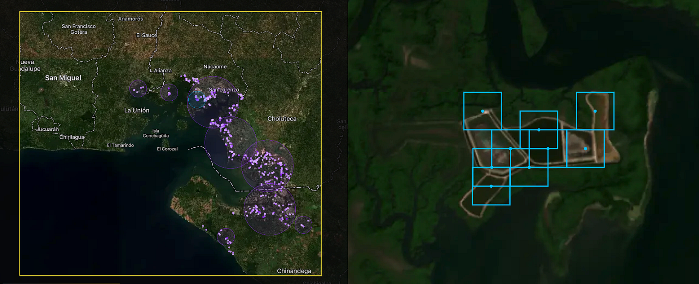
Here are some examples of how Earth Index is being used:
-
Combating Deforestation and Illegal Activities: In collaboration with Mongabay, Earth Index was used to pierce through dense canopy cover and identify hidden, illegal narcotrafficking airstrips in the Amazon. Similarly, the platform can rapidly locate illegal gold mining scars, like those devastating parts of the Yanomami Indigenous Territory, helping to quantify the scale of the problem and guide enforcement efforts.
-
Monitoring Resource Extraction: Radio Free Europe utilized Earth Index to identify over 1300 quarries across the Balkans, revealing that roughly half lacked proper permits, highlighting potential environmental damage and unregulated extraction. This approach can monitor fracking wellpads, rubber processing plants, or other industrial facilities.
-
Protecting Water Quality and Ecosystems: Earth Index can locate Concentrated Animal Feeding Operations near sensitive waterways to assess runoff risks or identify expansions of shrimp farming into vital mangrove ecosystems.
-
Tracking Agricultural Expansion: The tool helps monitor the conversion of natural habitats into agricultural land by searching for patterns associated with new clearings or specific crop types.
The Infrastructure Challenge: Searching Billions of Vectors Affordably
Generating 3.2 billion high-dimensional vectors is one challenge; hosting and searching them efficiently presents another significant hurdle. Earth Index needed a solution that could:
-
Handle Massive Scales: Searching billions of vectors requires specialized indexing and querying capabilities.
-
Integrate Seamlessly with Geospatial Data: Earth Index heavily relies on geospatial operations (like filtering results within specific administrative boundaries or proximity to rivers). This made PostgreSQL with PostGIS a natural and essential choice for their core database. Standalone vector databases often lack the rich geospatial features required.
-
Maintain Performance: Users need results relatively quickly for the platform to be effective for investigation and monitoring.
-
Control Costs: Storing and searching billions of vectors, especially if requiring vast amounts of RAM for purely in-memory indexes, can become prohibitively expensive for many organizations, particularly non-profits.
Earth Index needed a vector search solution that lived within their chosen PostgreSQL environment, could scale massively, perform well, and wouldn’t break the bank on hardware costs.
Why PostgreSQL Rocks for Planetary-Scale Vectors
While specialized vector databases exist, Earth Index faced a critical need: seamlessly integrating vector similarity search with rich geospatial data and operations. This is where PostgreSQL, combined with extensions, truly shines:
-
Unified Data Platform: PostgreSQL, especially with the powerful PostGIS extension, allowed Earth Index to keep their vector embeddings alongside their crucial geospatial metadata (tile locations, administrative boundaries, proximity to features like rivers). This avoids the complexity and potential synchronization issues of managing separate databases for vector search and relational/geospatial data.
-
Leveraging the Power of SQL & PostGIS: Earth Index could combine vector similarity searches with standard SQL filters and complex PostGIS spatial queries (e.g., “find vectors similar to this example within this specific national park boundary” or “near this river system”) all within a single query interface. Standalone vector databases often lack this mature geospatial query capability.
-
Maturity and Ecosystem: Building on PostgreSQL means inheriting its decades of development, renowned stability, robust tooling, and wide community support – essential for a mission-critical platform like Earth Index.
However, searching 3.2 billion vectors efficiently requires more than just standard PostgreSQL capabilities.
Why Earth Index Chose VectorChord for Performance and Affordability
While the PostgreSQL ecosystem provided the ideal foundation, achieving the required performance and affordability at the scale of 3.2 billion vectors presented a significant challenge. Earth Index needed a solution that could deliver speed without breaking the bank.
Finding the right balance of performance, cost, and integration was challenging. Hutch Ingold, CTO of Earth Genome, explains their considerations:
When we evaluated solutions for our 3.2 billion vectors – recognizing the rapidly evolving tech landscape – standard pgvector didn’t meet our performance requirements at that scale. Dedicated options like Qdrant posed difficulties: hosted versions were too expensive, and self-hosting clustered deployments on our Kubernetes infrastructure seemed insufficiently mature at the time. We also examined cloud services, such as Google’s Vertex AI Vector Search, but the list price of $237,000 per month for our dataset was simply prohibitive.
This is where VectorChord became the enabling technology:
-
Performance Beyond Vanilla PGVector: VectorChord delivers the necessary speed enhancements – up to 5x faster queries, 16x higher insert throughput, and 16x quicker index building – addressing the performance limitations encountered with standard pgvector at this massive scale.
-
Affordable Scale via Disk-Based Indexing: Critically, VectorChord’s optimized disk-based indexing (leveraging cost-effective SSDs) directly counters the prohibitive costs highlighted by the CTO. It avoids the massive RAM requirements of purely in-memory approaches and the exorbitant monthly fees of managed cloud vector services, making the 3.2 billion vector index financially feasible.
-
Native Integration & Scalability: As a PostgreSQL extension, VectorChord provided these benefits within their chosen database, requiring no infrastructure changes. It’s built to scale efficiently, handling the billions of vectors needed for Earth Index’s global monitoring platform while maintaining interactive performance.
VectorChord provided the crucial combination of high performance, massive scalability, and cost-effectiveness directly within the familiar and powerful PostgreSQL environment that Earth Index needed.
Earth Index: Technical Architecture and Setup
To manage its planetary dataset effectively and affordably, Earth Index built its backend on a cluster of three powerful AWS EC2 i8g.16xlarge instances, powered by the latest Graviton4 ARM processor and Nitro SSD. Each provides 512 GB RAM, 64 vCPUs, and 15 TB of NVMe storage, offering a solid foundation for both computation and disk I/O. This setup, costing around $12,000 per month, delivers massive cost savings compared to the estimated $237,000 monthly fee for a comparable managed cloud vector service, making the project economically viable. These instances run PostgreSQL enhanced with VectorChord and PostGIS, efficiently hosting both the vector data and other application components.
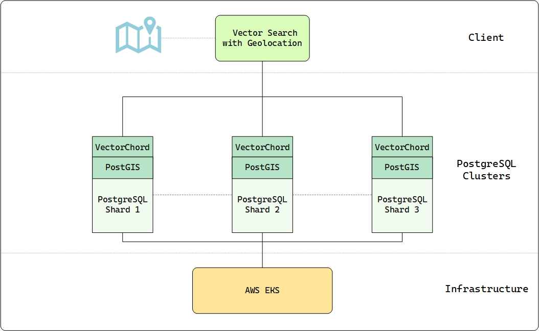
The core data resides in a partitioned table structure across the three nodes. The primary table, globe24, stores each tile’s unique ID, its geographic point geometry (geometry(Point, 4326)), a partition key (partkey), and the crucial 384-dimensional AI-generated embedding stored efficiently as halfvec(384). This sharding distributes the 3.2 billion rows across the cluster, allowing for parallel processing.
A key advantage of this architecture is the ability to perform complex, integrated queries. Earth Index commonly executes SQL statements that seamlessly combine VectorChord’s fast vector search (embedding <=> '{vector}'::vector) with PostGIS geospatial filtering (st_within(geom, '{geom}')) and partition pruning (partkey IN (...)). This allows users to find visually similar locations within specific geographic boundaries efficiently. Even with billions of vectors, this integrated approach yields practical performance, achieving a median query latency (p50) of approximately 761 ms for typical searches returning the top 500 results.
Enabling Environmental Action at Scale
By providing a cost-effective, scalable, and tightly integrated vector search solution within PostgreSQL, VectorChord helps enable Earth Index’s groundbreaking work. It allows them to manage their enormous “Planetary DNA” database affordably, ensuring that this powerful tool for environmental monitoring can reach the organizations and communities who need it most.
Join the Earth Index waitlist today to explore the environmental challenges in your neighborhood, understand your ecological footprint, and be part of a global effort to protect the planet.
We are thrilled to see Earth Index leverage VectorChord to turn satellite data into actionable environmental intelligence. Their success demonstrates the power of combining cutting-edge AI, robust database technology, and efficient vector search to address critical global challenges.
Interested in bringing large-scale vector search to your PostgreSQL database? Learn more about VectorChord or get started today!