This is the multi-page printable view of this section. .
VectorChord Engineering Blog & Releases
-
1: Engineering & Deep Dives
- 1.1: Scaling Vector Search to 1 Billion on PostgreSQL
- 1.2: How We Made 100M Vector Indexing in 20 Minutes Possible on PostgreSQL
- 1.3: Bringing Search‑Engine Ranking to PostgreSQL with VectorChord‑BM25
- 1.4: Optimize RAG with Contextual Retrieval in PostgreSQL
- 1.5: VectorChord: Cost-Efficient Upload & Search of 400 Million Vectors on AWS
- 1.6: All-in-one VectorChord Suite: Building Production-Ready RAG Solutions Directly in PostgreSQL
- 1.7: Introducing Vechord: Turn PostgreSQL into your search engine in a Pythonic way.
- 1.8: Beyond Text: Unlock OCR-Free RAG in PostgreSQL with Modal & VectorChord
- 1.9: 3 Billion Vectors in PostgreSQL to Protect the Earth
- 1.10: Vector Search Over PostgreSQL: A Comparative Analysis of Memory and Disk Solutions
- 1.11: PostgreSQL Full-Text Search: Fast When Done Right (Debunking the Slow Myth)
- 1.12: VectorChord-BM25: Introducing pg_tokenizer—A Standalone, Multilingual Tokenizer for Advanced Search
- 1.13: Hybrid search with Postgres Native BM25 and VectorChord
- 1.14: Vector Search at 10,000 QPS in PostgreSQL with VectorChord
- 1.15: VectorChord-BM25: Revolutionize PostgreSQL Search with BM25 Ranking — 3x Faster Than ElasticSearch
- 1.16: Do we really need a specialized vector database? (2023)
- 1.17: Supercharge vector search with ColBERT rerank in PostgreSQL
- 1.18: ARM + VectorChord: Affordable, Fast Vector Search
- 1.19: Why HNSW is Not the Answer
- 1.20: Benefits and Steps of External Centroids Building in VectorChord
- 1.21: VectorChord: Store 400k Vectors for $1 in PostgreSQL
- 1.22: Introducing PGVecto.rs Cloud - Scalable Vector Search in PostgreSQL, Now in the Cloud
- 1.23: Introducing Terraform Support for PGVecto.rs Cloud
- 1.24: Unleash the power of sparse vector
- 1.25: pg_bestmatch.rs: Elevate Your PostgreSQL Text Queries with BM25
- 1.26: My binary vector search is better than your FP32 vectors
- 1.27: pgvector vs. pgvecto.rs in 2024: A Comprehensive Comparison for Vector Search in PostgreSQL
- 1.28: Building LLM Applications in LangChain using pgvecto.rs
- 1.29: Building the RAG pipeline with LlamaIndex and pgvecto.rs
- 1.30: Do we really need a specialized vector database?
-
2: Release Notes
- 2.1: VectorChord 1.1: Native 4/8 Bit Vector Types and Per-Index Query Defaults
- 2.2: VectorChord 1.0: Developer-First Vector Search on Postgres, 100x Faster Indexing than pgvector
- 2.3: VectorChord 0.5: New RaBitQ-empowered DiskANN Index and Continuous Recall Measurement
- 2.4: VectorChord 0.4: Faster PostgreSQL Vector Search with Advanced I/O and Prefiltering
- 2.5: VectorChord 0.3: Bringing Efficient Multi-Vector Contextual Late Interaction in PostgreSQL
- 2.6: VectorChord 0.2: 60K-Dimensional Vectors, 50% Faster Indexing with ARM
- 2.7: pgvecto.rs 0.2: Unifying Relational Queries and Vector Search in PostgreSQL
1 - Engineering & Deep Dives
1.1 - Scaling Vector Search to 1 Billion on PostgreSQL
For teams trying to run vector search at billion scale themselves, the challenge is often not raw performance, but practicality. Many solutions designed for billion-scale, low-latency vector search come with practical constraints, requiring tradeoffs that affect how easily they can be adopted.
Most existing approaches fall into one of a few categories:
-
Operationally complex: Powered by multi-node distributed system that are difficult to manage, operate, and maintain over time.
-
Build-time prohibitive: Requiring long index build times, which makes re-indexing costly and easily impacts production workloads.
-
Memory heavy: Depending on up to 1 TB of memory on a single machine, making the hardware significantly less affordable for most teams.
These tradeoffs are visible in existing public benchmarks. For example, ScyllaDB reports up to 98% recall with a P99 latency of 12.3 ms on DEEP-1B, but this result depends on multiple large instances. YugabyteDB, on the same dataset, reports significantly higher tail latency, with P99 reaching 0.319 seconds at the same scale.
| Latency / Recall | Hardware | Build time | |
|---|---|---|---|
| ScyllaDB | 13ms / 98% | 3×AWS r7i.48xlarge + 3×AWS i4i.16xlarge |
24.4 h |
| YugabyteDB | 319 ms / 96% | Not reported | Not reported |
| VectorChord | 40 ms / 95% | AWS i7ie.6xlarge |
1.8 h |
For single-node deployments, previous work from Scalable Vector Search (SVS) shows that indexing DEEP-1B with HNSWlib typically requires 800 GiB of memory, though SVS or FAISS-IVFPQs can reduce it to around 300 GiB, which is still a substantial hardware requirement.

This makes smooth scaling difficult for teams that want to stay self-hosted. Moving from 1 million to 1 billion vectors often requires rethinking the architectures: new hardware assumptions or a different workflow.
With VectorChord 1.0.0, scaling is far more easy. By taking advantage of the new Hierarchical K-means and other optimizations, indexing 1B vectors follows the same process as indexing 1M vectors. This is exactly how we use it as well: Simply move to a slightly larger machine, for example from an AWS i7i.xlarge to an i7i.4xlarge.
The DEEP-1B Benchmark
To validate VectorChord’s capability at the billion-vector scale, we use the Yandex DEEP-1B dataset from BIGANN. DEEP-1B is a widely adopted benchmark for large-scale vector search, consisting of 1 billion 96-dimensional embeddings generated from deep learning models trained on natural images.
Because of its scale, DEEP-1B is widely used as a benchmark dataset for evaluating large-scale vector search systems. Its broad adoption makes results easy to reproduce and compare, particularly when assessing indexing performance, query latency, and resource efficiency at the billion-vector scale.
For such a huge dataset, building a VectorChord index requires:
-
Storage: Approximately 900 GB of high-performance SSD
-
Memory (shared_buffers): No less than 60 GB, managed by PostgreSQL
-
Memory (extra): At least 60 GB extra memory required during index construction
Based on these requirements, an AWS i7i.4xlarge is the minimum configuration for indexing at this scale. Our tests were run on an AWS i7ie.6xlarge, reflecting practical deployments where additional memory is provisioned to reduce disk access and maintain stable query latency.
| instance | AWS i7i.4xlarge |
AWS i7ie.6xlarge |
|---|---|---|
| Physical Processor | Intel Xeon Scalable (Emerald Rapids) | Intel Xeon Scalable (Emerald Rapids) |
| vCPUs | 16 | 24 |
| Memory (GiB) | 128 | 192 |
| Disk Space (GiB) | 3750 GB NVMe SSD | 2×7500 GB NVMe SSD |
| Price | $1088 monthly | $2246 monthly |
All experiments were run with VectorChord 1.0.0 on PostgreSQL 17. The SQL below is the exact command we used to build the index:
Here’s what each option does in our build configuration:
-
build.pin: Enables build-time pinning, caching the hot portion of the index in shared memory to speed up indexing on large datasets. -
residual_quantization: On DEEP-1B, we find that enabling residual quantization improves query performance, so we keep it on for this benchmark. -
build.internal.build_threads: Uses 24 threads for the K-means build stage, helping saturate available CPU resources on the instance. -
build.internal.lists: Based on our experience, we choose the appropriate list according to the number of rows. Using a two-level list helps significantly at large scale, improving both index build efficiency and query performance. -
build.internal.kmeans_algorithm.hierarchical: Enables the Hierarchical K-means path introduced in VectorChord 1.0, which significantly accelerates index construction at scale.
Our results
Index construction completed in 6,408 seconds (≈ 1.8 hours) when utilizing 24 CPU cores on a single AWS i7ie.6xlarge machine, demonstrating that billion-scale indexing can be completed within a practical window.
The figure shows query throughput versus recall on the Deep1B dataset using a single search thread, evaluated for both Top-10 and Top-100 queries, with all queries run against a warm cache.

For Top-10, throughput ranges from over 117 QPS at ~0.91 recall to around 69 QPS at ~0.95 recall. Top-100 queries follow the same pattern, with throughput decreasing as recall increases.
The table below lists the exact search parameters behind each data point, varying the number of probes while keeping epsilon = 1.9 fixed. Together, the figure and table show that even at the 1B-vector scale, VectorChord provides stable and tunable query performance on a single machine.
| probes / epsilon | Recall@Top 10 | QPS | P99 latency / ms |
|---|---|---|---|
| 40,120 / 1.9 | 0.9132 | 117.45 | 12.33 |
| 40,160 / 1.9 | 0.9305 | 97.32 | 14.61 |
| 40,250 / 1.9 | 0.9511 | 68.87 | 20.53 |
| probes / epsilon | Recall@Top 100 | QPS | P99 latency / ms |
|---|---|---|---|
| 40,180 / 1.9 | 0.9051 | 66.12 | 22.60 |
| 40,270 / 1.9 | 0.9318 | 49.55 | 30.40 |
| 40,390 / 1.9 | 0.9509 | 37.53 | 39.70 |
These results demonstrate that vector query performance can be practical and predictable on a single machine, even at the billion scale.
Summary
VectorChord 1.0.0 demonstrates that real-time vector search can scale cleanly from 1 million to 1 billion vectors without forcing users to change architectures, workflows, or usages. Whether you’re building image search, AI-powered applications, or RAG pipelines, VectorChord is designed to be a reliable vector engine that runs on your own machine, scaling naturally as your data grows.
Ready to scale up? You can get started today, or reach out to us on GitHub or Discord to learn more and get support from the community.
1.2 - How We Made 100M Vector Indexing in 20 Minutes Possible on PostgreSQL
1. Introduction
In the past few months, we’ve heard consistent feedback from users and partners: while our goal of providing a scalable, high-performance alternative to pgvector is well-received, index build time and memory usage remain major concerns at billion-scale.
Now VectorChord can index 100 million 768-dimensional vectors in 20 minutes on a 16 vCPU machine with just 12 GB of memory. By contrast, indexing the same data with pgvector requires around 200 GB of memory and about 40 hours on a 16-core instance. And pgvector with insufficient memory often suffer from page swapping, making builds even slower.
In short, memory usage and build time have become the key barriers to large-scale deployment of vectors. Through a series of targeted optimizations, we reduced build time to 20 minutes and memory usage by 7×, with only minor accuracy trade-offs.
With these improvements, we can now use far cheaper machines with much less memory, without a GPU, while still hosting 100 million 768-dimensional vectors:
| Instance | Price | Memory used / total | |
|---|---|---|---|
| Previous minimum | Amazon i7i.8xlarge | 🟨 $2174 monthly | 135 GB / 256 GB |
| Recommend for faster indexing | Amazon i7i.4xlarge | ✅ $1087 monthly | 12 GB / 128 GB |
| Minimum | Amazon i7i.xlarge + GPU for indexing | ✅ $272 monthly + GPU cost | 6 GB / 32 GB |
In the following sections, we will introduce how we optimized these phases to make index building faster and more memory-efficient. The optimizations are organized as follows: one targets each phase.
| Optimization | Target phase | Result |
|---|---|---|
| Hierarchical K-means ➕ Dimensionality Reduction | 1️⃣ Initialization | 🚀 30 min (GPU) → 8 min (CPU) 🧾 135 → 23 GB |
| Reducing Contention | 2️⃣ Insertion | 🚀 420 min → 9 min |
| Parallelize Compaction | 3️⃣ Compaction | 🚀 8 min → 1 min |
2. Background
The index type used in VectorChord, vchordrq is logically a tree of height \(n+1\). The first \(n\) levels of the tree are immutable which serve purely as the routing structure for search. The \((n+1)\)-th level stores all data.
If \(n=1\), the index is a flat, non-partitioned structure. If \(n=2\), it is an inverted file index. If \(n=3\), it has an additional layer.

The index building can be divided into 3 phases: Initialization, insertion and compaction.
-
Initialization Phase
In this phase, top \(n\) levels of the tree are written to the index. Firstly, the index samples vectors in the table. Then the index builds the tree by clustering the samples, the centroids, the centroids of centroids, and so on for \(n\) levels. Finally the tree is written to the index. -
Insertion Phase
The index inserts vectors from the table into the bottom level of the tree. -
Compaction Phase
The index converts all the inserted vectors from non-compact layout to compact layout.
3. Making Clustering Faster and More Memory-efficient
In the past, although we can build index for 100 million vectors on small instances, it typically needs a GPU to accelerate clustering.
The main bottleneck in the initialization phase is clustering, which is time-consuming and memory-intensive. In fact, it decides the minimum memory requirement of index building. If we implement clustering on the CPU in a way that is both fast and memory-efficient, it would be practical to build indexes on small instances without large memory and GPUs.
Let \(n\) be the number of vectors, \(c\) be the number of centroids, \(d\) be the dimension of vectors, and \(l\) be the number of iterations. The time complexity of K-means is \(O(ncdl)\), and the space complexity of it is \(O(nd + cd)\). Let \(f\) be the sampling factor, in other words, \(n=fc\). The time complexity of K-means is \(O(fc^2dl)\), and the space complexity of it is \(O(fcd)\).
In the following sections, we will explain how to reduce the complexity, as well as decrease \(d\) and \(f\) for better performance.
Hierarchical K-means
Constrained by time complexity, K-means cannot be improved beyond linear speedup, regardless of the optimizations applied. Even on a GPU, this would take 30 minutes. So we must reduce time complexity.
A simple idea is to divide the samples to multiple disjoint subsets, run K-means on every subset, and then merge the centroids on every subset. To balance the size of these subsets and the number of them, we choose \(\sqrt{c}\) as the number of subsets. In order to generate \(\sqrt{c}\) subsets, we initially perform a small-scale K-means and then assign the \(n\) vectors to \(\sqrt{c}\) disjoint subsets using \(\sqrt{c}\) centroids.
Assuming the subsets are of uniform size, the time complexity of this step is \(O(f\sqrt{c}\sqrt{c}dl) \times \sqrt{c} = O(fc^{1.5}dl)\). If f = 64 and c = 160,000, the algorithm would be roughly 400 times faster.
There is still a small problem here. How many centroids should be computed for a subset? If we ignore the constraint that it must be an integer, it’s \(\frac{n}{|s|}c\). Considering this constraint, this problem is similar to proportional representation, where Sainte-Laguë method is an algorithm that minimizes the average seats-to-votes ratio deviation. It works as follows.
After all the votes have been tallied, successive quotients are calculated for each party. The formula for the quotient is \(\frac{V}{s_i+0.5}\), where \(V\) is the total number of votes that party received, and \(s_i\) is the number of seats that have been allocated so far to that party, initially \(0\) for all parties.
Now clustering on CPU is practical. However, this algorithm does not reduce memory usage.
Dimensionality Reduction
It’s time to review the 140 GB of memory used for K-means samples. It would definitely result in OOM on a machine with memory of 128 GB. Consider the space complexity \(O(fcd)\), we have two ways to reduce memory usage: reduce \(f\), and reduce \(d\).
Let’s reduce \(d\) now. Although it sounds incredible, we can first reduce the dimension of the vectors and then perform clustering without compromising accuracy. Christos’s results show that running K-means on low-dimensional projections can still maintain good accuracy.
Johnson–Lindenstrauss lemma states that a set of points in a high-dimensional space can be embedded into a space of much lower dimension in such a way that distances between the points are nearly preserved. In the classical proof of the lemma, the embedding is a random orthogonal projection.
According to the theorem, \(n\) vectors can be reduced to \(O(\lg n)\) dimensions. Specifically, we only need to construct a random Gaussian matrix, which allows us to reduce high-dimensional vectors to low-dimensional ones using matrix multiplication. Then we perform K-means on it.
Since we need to reduce memory usage, we apply the Johnson-Lindenstrauss transform directly during sampling. In the end, we obtain low-dimensional centroids. We do not attempt to perform an inverse transform; instead, we sample from the table again, find the nearest cluster in the low-dimensional space after the Johnson-Lindenstrauss transform, and thereby recover the high-dimensional centroids.
With dimensionality reduction from 768 to 100, the resident set size of the instance dropped to 23 GB, allowing us to build the index on an i4i.xlarge instance. Additionally, this also results in clustering being 7 times faster, in theory. With hierarchical K-means and dimensionality reduction, the time of initialization phase fell to 24 minutes.
Reducing \(f\) is trivial. It’s configured as build.internal.sampling_factor so we only need to change the configuration. Let’s set \(f\) to \(64\). The resident set size of the instance dropped to 6 GB, and clustering is roughly 2 times faster.
Sampling
In order to perform clustering, we need to sample vectors from the table. Our previous approach, reservoir sampling was reliable but slow. This method is used because we do not know the number of rows in the table without doing a full table scan. However, it would still perform a full table scan.
To avoid a full table scan, we take advantage of PostgreSQL table access method’s sampling interface. The interface takes a function that, given the maximum block number, produces an iterator of block numbers. The interface then returns an iterator over the tuples in those blocks. In order to generate such a random iterator, we can generate an ordered sequence and perform Fisher–Yates shuffle on it, but this consumes memory. In fact, we have a more clever approach. In cryptography, a pseudorandom permutation is a function that cannot be distinguished from a random permutation.
Feistel network could be used as a pseudorandom permutation. It defines as \(L_{i + 1} = R_{i}, R_{i + 1} = L_{i} \oplus F(R_i, K_i)\), where \(F\) is a hash function, \(K_i\) is the random seed. The input of the function is \((L_0, R_0)\), and the output of the function is \((L_n, R_n)\). So it’s a function from \([0, 2^n) \times [0, 2^n)\) to \([0, 2^n) \times [0, 2^n)\). Cleverly, because of \(R_{i} = L_{i + 1}, L_{i} = R_{i + 1} \oplus F(L_{i + 1}, K_i)\), this function is reversible. A reversible function is bijective, so this function is bijective. \([0, 2^n) \times [0, 2^n)\) is equivalent to \([0, 4^n)\), and therefore it’s a permutation of \([0, 4^n)\). Now, by filtering out all elements greater than the maximum block number from this permutation, we get the lazy random permutation we need.
Based on the interface and this function, we implement block sampling, which only needs to access the sampled vectors.
With all these optimizations, the initialization phase takes only 8 minutes in total now.
4. Reducing Contention
In earlier experiments, building the index for the LAION-100m dataset on an Amazon i7i.16xlarge (64 vCPU) instance takes approximately 420 minutes during the insertion phase if \(n=2\) is used, and this is entirely computation-bound.
Starting with version 0.1, VectorChord allows \(n\) to be set to a positive integer no greater than \(8\). From our perspective, it is necessary for billion-scale data. However, at that time, we didn’t actually know how much fast it would be.
After trying \(n=3\) on a smaller instance, i7i.4xlarge (16 vCPU), we observed that the insertion phase completed in just 40–60 minutes. At that point, CPU utilization stayed around 40%, and IO throughput fluctuated between 300 MB/s and 800 MB/s, suggesting a large room for optimization.
Reducing Linked-List Contention
The insertion phase took 40–60 minutes. Surprisingly, our tests showed that 8 workers took 40 minutes, while 16 workers took 55 minutes. This suggests the existence of potential contention among workers during insertion.
In the implementation, the index maintains a single linked list to store full-precision vectors aside from the tree, while the tree only stores quantized vectors. This makes the tree nodes much smaller and allows the tree to fit in memory.
Since changing \(n\) from \(2\) to \(3\), the number of computations of insertion phase has decreased. As a result, inserting vectors into this linked list occurs much more frequently. Parallel workers experience contention when inserting into the list. So more workers actually slow down the insertion, making the performance unpredictable.
To address this, we replaced the single linked list with \(1+k\) linked lists. The first linked list stores full-precision vectors for the top \(n\) levels of the tree, while the other \(k\) lists store vectors for the bottom level. During index build, the \(i\)-th worker inserts vectors into the \((i\ \text{mod}\ k)\)-th list. We set \(k=32\) as the default, and consider it sufficient for most cases.
With this change, CPU utilization stabilizes around 54%, and the insertion phase now completes in about 30 minutes.
Reducing Page Extension Lock Contention
The CPU utilization still suggested that more optimizations were potential. But where exactly was the bottleneck? We started our investigation by checking PostgreSQL worker processes using htop.

Many processes showed waiting on their titles, indicating heavy internal contention inside PostgreSQL. Searching in the code, we traced the source that sets waiting to lock.c. To measure off-CPU time, we turned to offcputime from BCC. Then, with stackcollapse.pl and flamegraph.pl from Brendan Gregg’s FlameGraph, we generated a flame graph for the process’s off-CPU time.

The result was surprising: the culprit was LockRelationForExtension, which acquired the lock of the index for extending it.
Here, the ockRelationForExtension should be LockRelationForExtension. This may be result from an unknown behavior from the flamegraph.pl script.
Why does acquiring this lock become a bottleneck? Searching through the PostgreSQL mailing list led us to this discussion.
In short, PostgreSQL places a lock on each index to prevent this index from being extended concurrently. But the granularity of this lock is too coarse. Thanks to Andres Freund, a patch was introduced that narrows the critical section and fixes the issue, but it requires the new API available since PostgreSQL 16.
Since VectorChord supports PostgreSQL 13 through 18, we took advantage of the old API in the early development. Unfortunately, that meant we overlooked this optimization.
After switching to the new API, the insertion phase dropped to 22 minutes.
Bulk Page Extensions
However, another round of profiling revealed that the bottleneck remains in the same area.

As the critical section of the lock is already narrowed, we need to speed up the page extension to ease the bottleneck. Extending a file using fallocate is fast on the filesystem. If fallocate is used for extending the index, the average time for extending a page will be shorter. So the question becomes: can we use fallocate to extend the index?
The answer is yes. If the index is extended more than 8 pages at a time, PostgreSQL automatically switches from pwrite to fallocate. By requesting 16 pages at once, we significantly increased the speed of page extension.
With this change, the insertion phase dropped to 9 minutes, CPU utilization stabilized at 90%, and write throughput stayed around 1.8 GB/s. iostat reported IO utilization of 0.75–0.85, indicating we were finally making better use of the resources.
There is still room for improvement. But for now, there is no longer any trivial bottleneck in the insertion phase.
5. Parallelize Compaction
On the bottom level of the tree, quantized vectors exist in two layouts:
-
Non-compact layout (insert-oriented): Every quantized vector is stored as a tuple, so data can be appended directly without modifying existing tuples.
-
Compact layout (search-oriented): Every 32 quantized vectors are stored as a tuple. It’s optimized for SIMD and makes the search fast.
All vectors are initially inserted in the non-compact layout, and will be converted into the compact layout in the final phase. It is worth noting that this phase is serial and takes about 8 minutes during index build.
Since the other phases have become much faster, optimizing this phase has become more important. So we parallelize this phase. If there are \(k\) workers, and \(m\) nodes in the level \(n\) of the tree, the children of the \(i\)-th node will be compacted by the \((i\ \text{mod}\ k)\)-th worker. Benefiting from parallelism, the compaction phase now takes less than 1 minute.
You may notice that an effective index also requires this compaction occasionally to maintain search performance. PostgreSQL has a vacuum mechanism for this purpose. So this phase is also performed for the indexes routinely in vacuum. Unfortunately, we cannot parallelize it in vacuum: PostgreSQL does not allow an index to use nested parallelism. If the vacuum is parallel, the index could not start parallel workers again.
6. Conclusion
Previously, indexing the LAION-100M dataset with VectorChord 0.5.3 on an Amazon i7i.4xlarge instance was infeasible due to out-of-memory (OOM) failures. Offloading clustering to a GPU made the build possible, yielding a recall of 95.6% at 120 QPS for querying the top 10 results, with a build time of 30 minutes on the GPU and 420 minutes on the i7i.4xlarge.
With the optimizations introduced in VectorChord 1.0.0, the index can now be built entirely on the i7i.4xlarge instance in only 18 minutes, achieving a recall of 94.9% under the same QPS setting.
Our goal is to make VectorChord one of the best ways to do retrieval on PostgreSQL, from the first prototype to billion‑scale datasets. If you’re already using pgvector, we’d love you to try VectorChord 1.0 on your real workloads and tell us where it helps and where it can do better.
1.3 - Bringing Search‑Engine Ranking to PostgreSQL with VectorChord‑BM25
Modern applications rely on PostgreSQL for its fully ACID‑compliant, expressive SQL, and rich ecosystem of extensions. The database handles relational workloads exceptionally well, but many projects also need to search for large text collections—product descriptions, support tickets, documentation—and present the most relevant rows first. PostgreSQL’s native tools offer a foundation for this, yet their default ranking logic can leave ideal matches buried under less useful results. VectorChord‑BM25 changes that equation by introducing the BM25 relevance‑scoring algorithm directly into PostgreSQL.
What is PostgreSQL?
PostgreSQL is an open‑source, enterprise‑class relational database management system (RDBMS) renowned for reliability, data integrity, and standards compliance. It supports advanced features such as window functions, materialized views, JSONB storage, and a robust extension mechanism that allows developers to add capabilities. Learn more about PostgreSQL here.
Full‑Text Search with tsvector
PostgreSQL has its own tool for basic text search called tsvector. Think of it as a special column that stores the important words (lexemes) from each document in a way the database can search quickly. When you add a GIN or GiST index on that column, PostgreSQL can find rows that match a keyword almost instantly. You write searches with the @@ operator, and the full details are in the PostgreSQL manual here.
Where native ranking falls short
While the ts_rank function can sort matches, its scoring method is basic. Long documents that mention a term once may outrank short documents focused entirely on the query, and rare but important words carry little extra weight. In large datasets, the perceived relevance of results often suffers.
What’s New: VectorChord Adds BM25
VectorChord‑BM25 is a lightweight PostgreSQL extension that augments the existing text‑search stack with the industry‑standard BM25 ranking formula. Instead of exporting data to an external search engine, you can keep everything inside a single database, gaining:
-
Ranking that rewards distinctive terms and penalises irrelevant verbosity
-
In‑index scoring, reducing query latency
-
Seamless SQL workflow—documents remain rows, searches remain queries
What is BM25?
BM25 (Best Matching 25) is a probabilistic retrieval model widely adopted by search engines and academic literature. It evaluates how often a query term appears in a document, how rare that term is across the entire corpus, and how long each document is. The algorithm is discussed in detail on its Wikipedia page, but the core idea is straightforward:
-
Term Frequency (TF) – More occurrences of a word in a document increase its relevance but with diminishing returns.
-
Inverse Document Frequency (IDF) – Rare words are more informative than common ones.
-
Document Length Normalisation – Shorter documents aren’t unfairly penalised when they focus on the query topic.
VectorChord implements BM25 through a new index type and operator (<&>), letting PostgreSQL compute scores while scanning the index.
Two Practical Examples
Below are concise demonstrations that illustrate how to adopt VectorChord‑BM25 with a pre‑trained tokenizer and, for specialised domains, with a custom model.
Example 1: Quick Start with a Pre‑Trained Model
The query returns rows already ranked by BM25, producing more intuitive results than the default ts_rank.
Example 2: Custom Model for Domain‑Specific Vocabulary
Domain‑specific text—medical notes, legal briefs, technical logs—often includes jargon absent from general models. VectorChord lets you train a custom tokenizer directly in SQL.
With a tailor‑made vocabulary, the database recognises abbreviations such as “OOM” and “Kubernetes,” yielding more precise rankings for technical support scenarios.
Final Thoughts
VectorChord‑BM25 brings search‑engine quality relevance to the PostgreSQL ecosystem without introducing an additional service layer. By combining flexible tokenization, an efficient BM25 index, and familiar SQL, it enables developers to deliver significantly better search experiences while preserving the operational simplicity of a single database system. If your application relies on PostgreSQL and demands accurate text ranking, VectorChord‑BM25 is well worth exploring.
1.4 - Optimize RAG with Contextual Retrieval in PostgreSQL
In the standard approach to Retrieval Augmented Generation (RAG), a common practice is to break down large documents into smaller, more manageable chunks. This is primarily done to improve the efficiency of the retrieval process, leveraging the sentence embedding and keyword bm25 scoring, allowing systems to quickly find and pull relevant pieces of information. While effective in many scenarios, this method can introduce a significant challenge: the potential for individual chunks to lose their surrounding context.

An example could be from a collection of historical documents. If a user asks about a specific event, and a retrieved chunk says: “The treaty was signed, bringing an end to hostilities.”
Without the surrounding text, this chunk lacks vital context such as which treaty was signed, who the involved parties were, and when or where this significant event took place. Relying solely on this decontextualized snippet would provide an incomplete and potentially inaccurate picture to the LLM, hindering its ability to generate a comprehensive and accurate answer about the historical event.
The example highlights that while chunking aids retrieval efficiency, it can inadvertently strip away the necessary context that gives meaning and relevance to the individual pieces of information. This loss of context can significantly impact the quality and accuracy of the responses generated by LLMs in a RAG system.
To tackle this problem, Anthropic explores a method called Contextual Retrieval.
Basically, it could be treated as the chunk augmentation with the document context.

This article will walk through the steps to improve the retrieval accuracy with the help of contextual information. We use the same prompt, dataset, and metrics described in the anthropic tutorial. Note that we use a different embedding model and LLM in this experiment, so the results will differ. However, this does not reflect the model’s accuracy, as the dataset consists of code rather than natural language.
We mainly use Gemini models to generate the chunk context and text embedding, other models also work. The embedding quality affects the vector retrieval metrics heavily, we recommend checking the leaderboard to find the one that suits your use case. For the keyword tokenization, we use the default BERT tokenizer, you can also try other solutions.
The rerank part is not the main point of this article, if you want to know more about the rerank methods, check our article about the cross-encoder rerank and token-level late interaction rerank. BTW, since we support multivector MaxSim index, the token-level late interaction rerank can be done more efficiently.
Prepare the environment
We provide both vector search and keyword search features in our VectorChord-suite docker image.
We will use the vechord Python library to reduce the boilerplate code and simplify the process.
Define the RAG-related tables
Let’s get started with the basic RAG process.
This includes the vector embedding index and keyword index.
To load the datasets:
Evaluation
Now we have everything for the basic RAG process. Let’s define the evaluation metric Pass@k , which means that retrieved top-k chunks contain how many of the groundtruth chunks.
We can try different retrieval strategies like vector search, keyword search, hybrid search with fusion or rerank.
Those strategies can be defined as:
Contextual retrieval
The LLM generates contextual information with the prompt like:
The prompt above is a general one designed for retrieval tasks. You may find that a more specialized prompt offers better performance for your specific use case.
This feature is already included in the vechord library.
GeminiAugmenter also supports the prompt caching like Claude, but it requires the cached content to be at least 32768 tokens, which is not the case for this dataset.
Then, we can expand the strategies like:
Benchmark
topk=5
| Pass_at_5 | QPS | |
|---|---|---|
| vector search | 0.8071 | 289.024 |
| keyword search | 0.7003 | 337.211 |
| vector contextual search | 0.8404 | 307.253 |
| keyword contextual search | 0.8033 | 331.239 |
topk=10
| Pass_at_10 | QPS | |
|---|---|---|
| vector search | 0.8574 | 254.730 |
| keyword search | 0.7577 | 219.653 |
| vector contextual search | 0.8807 | 247.819 |
| keyword contextual search | 0.8563 | 216.560 |
All the code can be found in our vechord repository.
1.5 - VectorChord: Cost-Efficient Upload & Search of 400 Million Vectors on AWS
In this article, we will describe one method for uploading, indexing, and searching a big dataset of vector data in a cost-efficient manner using the real-world LAION-400M dataset and the VectorChord extension in PostgreSQL.
We’re attempting to show you what kind of hardware setup you need to allow you to search through this vast dataset using VectorChord. We want to make sure that you have a good experience with a search that is both accurate and fast.
VectorChord is a PostgreSQL extension that may bring high-performance vector database capabilities directly into your PostgreSQL database with high compatibility with the popular pgvector extension’s interface where possible.
The version of VectorChord to be used for this tutorial must be v0.3.0 or later. While VectorChord is compatible with most of the recent pgvector versions, pgvector 0.8.0 was extensively tested.
Dataset
The dataset used for this experiment is LAION-400M, which is a dataset with approximately 400 million vectors derived from images. Each vector is 512-dimensional and was generated from a CLIP model.
The total vector data is approximately 400 GB. The vectors have been normalized, so it is feasible to use multiple distance measures (L2, cosine, dot product). To be consistent with other benchmarks on this dataset and following the nature of CLIP embeddings, we employed the cosine distance measure in this experiment.
LAION-400M is divided into 409 chunks, each containing around 1 million vectors. We will process these chunks sequentially for uploading.
Algorithm
Searching through 400 million vectors is a huge challenge, especially as the data size means much of it must live on disk rather than in memory. We need algorithms built for this scale! A popular and effective method for handling large, disk-based vector data is the graph-based DiskANN, known for its Low memory and resource cost.
However, being derived from HNSW, DiskANN also has some inherited disadvantages:
-
Slow index building: For large scale datasets, it’s well known that building indexes with DiskANN can take a long time.
-
Poor insert performance: For streaming inserted vectors, updating a graph-based index requires traversing the partial graph. This is even more costly because DiskANN’s on-disk graph must be loaded into memory.

VectorChord addresses these problems with its VChordRQ index, which combines a cluster-based index (ivf) with a clever data compression scheme called RabitQ. In addition to better precision and latency in both memory and disk, RabitQ’s strength lies in its strong theoretical guarantee of accuracy, which is different from other compression techniques. This helps us achieve an excellent trade-off between accuracy and efficiency!
For more comparisons with VChordRQ(VectorChord), HNSW(pgvector) and StreamDiskANN(pgvectorscale), please see our previous blog.
Hardware
Based on our experiments, we determined the following cloud instance type to be sufficient to index and query the dataset with acceptable latency:
-
Instance Type: AWS EC2 i8g.2xlarge ($501.0720 / month)
-
CPU: 8 vCPUs (ARM64)
-
RAM: 64GB
-
Storage: 1875 GB NVMe SSD
This configuration provides the necessary compute and ample fast local NVMe storage. The 64GB of RAM serves as cache to accelerate search queries.
We used an instance with 1875 GB NVMe storage, though only about 1014 GB was needed. This was the minimum AWS option providing sufficient fast local SSD. Finding a machine with less storage could reduce costs.
For the PostgreSQL setup within this instance, we adjusted the shared_buffers parameter:
-
Set to 48GB during the index building process.
-
Increased to 54GB for search evaluation to allow more data caching for search performance.
Uploading and Indexing
The VectorChord VChordRQ index uses an Index-based Vector File (IVF) structuring. While VChordRQ can compute the required centroids during the index building process, the building of an index of this size (400M vectors) pre-calculating the centroids out of the system significantly accelerates the process of building an index.
For LAION-400M, we performed an external k-means clustering step to determine these centroids. This was done on an instance with an A10 GPU for faster computation.
-
The clustering was configured for
nlist = 160000clusters. -
The clustering took approximately 220 seconds per iteration for 25 iterations, totaling about 1.5 hours.
Once we have computed the centroids, we set up the VectorChord-enabled PostgreSQL database. We used a pre-built Docker image for convenience:
This Docker image contains PostgreSQL 17 with pgvector 0.8.0 and VectorChord 0.3.0 installed.
The core of the upload process involves inserting the pre-computed centroids into a dedicated table and then inserting the vectors from the LAION dataset chunks into the main data table. This can be done efficiently using a client library like psycopg in Python with batched inserts.
First, insert the centroids into a table (e.g., laion_centroids):
Then, insert the vectors from the dataset into the data table (e.g., laion):
After inserting all data, we build the VectorChord index (vchordrq). vchordrq stands for RabitQ, which is VectorChord’s highly optimized index type based on the IVF structure combined with quantization and efficient reranking.
The image below shows the system resource utilization (CPU, memory, and disk usage) on the instance during the upload and indexing process. The disk usage graph shows the data being written (initial steep increase) and the subsequent index building (steady increase), resulting in a final size over 1TB. The CPU and memory graphs indicate the resources consumed throughout this process.

Ground Truth Data
To correctly measure search performance and accuracy, comparing to ground truth is vital. The LAION data set comes without inherent ground truth. We are in debt to the Qdrant team for having published the ground truth data they had prepared for their tutorial on this dataset.
Their methodology involved performing a full-scan nearest neighbor search for the first 100 vectors in the dataset to find the top 50 true nearest neighbors for each query. We used this same exact ground truth file to evaluate the VectorChord search accuracy.
Search Query
VectorChord search employs two main parameters to control the performance-accuracy trade-off: nprobe and epsilon.
-
nprobe: Configured using the
vchord.probessetting. This parameter determines how many clusters (partitions) of the IVF index are searched in the initial phase. A higher nprobe increases the search scope, potentially finding better results but also increasing latency. -
epsilon: Configured using the
vchord.epsilonsetting. This parameter controls the reranking precision. After fetching the initial candidates from the nprobed clusters, VectorChord performs a reranking step using more precise vector data. A larger epsilon means more candidates are considered and potentially reranked for higher recall, impacting latency.
These parameters are set as PostgreSQL session variables before executing the search query:
The ORDER BY embedding <=> '[...]' clause leverages the index to find the approximate nearest neighbors based on the specified distance metric (cosine distance, like CLIP). The LIMIT 50 retrieves the top 50 results.
Running Search Requests
After the index built is finished, we ran queries over the 100 ground truth vectors with varying nprobe and epsilon settings to try out performance versus precision trade-offs.
We expressed search latency in milliseconds (ms). “Cold” latency refers to instances where vector data of interest may need to be read from disk, while “warm” latency implies that data will be in memory.
Here are the average latencies and corresponding Precision@50 scores across the 100 queries:
| nprob / epsilon | Cold Latency (ms) | Warm Latency (ms) | Precision@50 |
|---|---|---|---|
| 10 / 0.8 | 112.5 | 7.0 | 0.8192 |
| 100 / 0.8 | 194.2 | 15.0 | 0.9216 |
| 200 / 1.0 | 331.2 | 24.9 | 0.9438 |
| 400 / 1.5 | 970.9 | 51.6 | 0.9608 |
| 800 / 1.9 | 2174.0 | 2174.0 | 0.9662 |
The table clearly illustrates the trade-off:
-
Increasing
nprobeandepsilongenerally leads to higher Precision@50. -
However, this comes at the cost of increased search latency, especially noticeable in cold scenarios where more disk I/O is required to fetch data from more clusters and perform more extensive reranking.
-
Warm cache performance is significantly faster, highlighting the importance of sufficient RAM for caching frequently accessed data.
-
It is possible to have over 90% precision through warm latencies less than 50ms, and increasing precision above this yields hundreds of milliseconds or even more than a second latency for best recall, depending on the parameters selected.
The graph below shows the trade-off between Queries Per Second (QPS) and Precision@50 for VectorChord (cold and warm cache) alongside Qdrant, with Qdrant’s metrics taken from their published benchmarks on a comparable 8 vCPU, 64 GB machine rather than run on the same hardware.

Conclusion
In this tutorial, we illustrated how VectorChord as an extension to PostgreSQL can be utilized to upload, index, and search a gigantic 400 million vector dataset cost-efficiently on relatively small hardware with fast NVMe SSD.
By using the VectorChord VChordRQ index with external centroids, we were able to handle the scale. Having carefully set nprobe and epsilon at query time provides precise control over the critical trade-off between search speed and accuracy, allowing users to tune the system to their specific needs.
VectorChord’s compatibility with the pgvector interface simplifies adoption for current pgvector users, and its vchordrq index provides powerful capabilities for large-scale vector search directly within the robust and familiar PostgreSQL environment.
1.6 - All-in-one VectorChord Suite: Building Production-Ready RAG Solutions Directly in PostgreSQL
Retrieval-Augmented Generation (RAG) is revolutionizing our interaction with vast datasets and language models. RAG systems offer more precise, contextually aware, and current answers by retrieving pertinent information before generating responses. Nonetheless, constructing robust, scalable, and efficient RAG pipelines poses considerable challenges, particularly for production use.
Many solutions feature complex architectures, using distinct databases for vector search, keyword search, and primary data storage. This commonly results in data synchronization challenges, greater infrastructure complexity, and higher operational costs.
What if you could build a powerful, production-ready RAG system directly within your trusted PostgreSQL database?
Enter the VectorChord Suite, a collection of PostgreSQL extensions designed to bring high-performance vector search, native BM25 ranking, and flexible tokenization capabilities right into Postgres. Let’s explore the components and how they enable next-generation RAG solutions.
What is the VectorChord Suite?
The suite comprises three key PostgreSQL extensions working in concert:
-
VectorChord: The core vector search engine. It’s specifically designed for scalable, high-performance, and disk-efficient vector similarity search within PostgreSQL.
-
VectorChord-bm25: This extension implements the sophisticated BM25 ranking algorithm directly inside PostgreSQL, leveraging efficient Block-WeakAnd algorithms. BM25 is a standard for relevance ranking based on keyword frequency and document characteristics.
-
pg_tokenizer.rs: Provides essential text tokenization capabilities needed for effective full-text search, enabling fine-grained control over how text is processed for full-text search.
By combining these extensions, you unlock powerful capabilities for building advanced RAG systems entirely within PostgreSQL.
How to Use the VectorChord Suite
You can use the tensorchord/vchord-suite image to run multiple extensions which are provided by TensorChord. The image is based on the official Postgres image and includes the following extensions:
Use Cases for the VectorChord Suite
Use Case 1: Powerful Hybrid Search with Native BM25 and VectorChord

In the RAG era, effective retrieval is paramount. Neither keyword search nor vector search alone is perfect:
-
Keyword Search (like BM25): Excels at precision, finding documents with exact keyword matches. It’s great for structured queries and term-specific searches. However, it struggles with synonyms, paraphrasing, and understanding the underlying meaning or semantic intent. (Leverages
VectorChord-bm25andpg_tokenizer). -
Vector Search: Captures deep semantic meaning and relationships between concepts, allowing it to find relevant information even if the exact keywords aren’t present. However, it can sometimes lack precision for queries demanding specific term matches. (Leverages
VectorChord).
The Solution: Hybrid Search. By combining the strengths of both approaches within Postgres, the VectorChord Suite bridges this gap. You can run a query that leverages:
-
VectorChord-bm25(powered bypg_tokenizer) for keyword precision. -
VectorChordfor semantic understanding.
The results from both can be intelligently combined (e.g., using reciprocal rank fusion - RRF or Model-based rerank) to produce a final ranking that is more accurate, contextually relevant, and semantically aware than either method could achieve alone. This delivers significantly better retrieval performance for your RAG applications.
Use Case 2: Beyond Text - OCR-Free RAG with ColQwen2 & VectorChord
Building RAG systems for documents like PDFs or scanned images often involves cumbersome pre-processing pipelines. Traditional methods rely heavily on Optical Character Recognition (OCR) and layout analysis to extract text. This process can be:
-
Slow: OCR can be computationally expensive.
-
Error-Prone: OCR accuracy varies significantly depending on document quality.
-
Lossy: Crucial visual contexts like tables, figures, formatting, and relative positioning is often lost during text extraction.
The Solution: OCR-Free, Visually-Aware RAG. What if you could query documents based on how they look and their content, without explicit OCR?
This is now achievable by combining:
-
Multi-Modal Vision Language Models (VLMs): Models like ColQwen2 can process images (document pages) and generate embeddings that capture both textual content and visual layout information.
-
VectorChord’s Multi-Vector Capabilities: VectorChord can efficiently store and search multiple vectors per document within Postgres – allowing you to store embeddings representing different aspects (e.g., text content, visual layout).
With this setup, you can query your document database using prompts that reference visual elements (“Find documents with a bar chart comparing sales figures”) or combined textual and visual cues, directly within PostgreSQL. This simplifies your RAG stack, potentially boosts retrieval accuracy by preserving visual context, and eliminates the bottlenecks associated with traditional OCR pipelines.
Why Build RAG in PostgreSQL?
Leveraging the VectorChord Suite within Postgres offers significant advantages:
-
Unified Data: Keep your source data, text, metadata, and vector embeddings all in one place.
-
Reduced Complexity: Eliminate the need for separate vector databases and synchronization pipelines.
-
Leverage Existing Infrastructure: Utilize your existing Postgres expertise, tooling, and operational practices.
-
Transactional Integrity: Benefit from PostgreSQL’s robust ACID compliance.
-
Rich Ecosystem: Access the wide array of tools and features available within the Postgres ecosystem.
Conclusion
The VectorChord Suite transforms PostgreSQL into a powerful, production-ready platform for building advanced RAG solutions. By integrating high-performance vector search (VectorChord), sophisticated keyword ranking (VectorChord-bm25), and flexible text processing (pg_tokenizer), you can implement cutting-edge techniques like hybrid search and OCR-free multi-modal retrieval directly within your database. Simplify your architecture, enhance retrieval accuracy, and unlock the full potential of RAG with VectorChord in PostgreSQL.
Previous Blog Post
In our previous blog, we shared some user cases where all images can be replaced with VectorChord Suite image.
References
1.7 - Introducing Vechord: Turn PostgreSQL into your search engine in a Pythonic way.
Today, we’re thrilled to announce the release of Vechord, a new Python library designed to dramatically simplify building robust search infrastructure directly on top of the PostgreSQL database.
In the rapidly evolving world of AI and large language models (LLMs), Retrieval-Augmented Generation (RAG) and semantic search have become crucial components. However, setting up the necessary vector search infrastructure often involves learning new database technologies, managing complex integrations, or wrestling with intricate frameworks. This adds friction and slows down development, especially for teams already comfortable with PostgreSQL.
The Challenge: Hybrid Search Complexity
Building search capabilities often means:
-
Choosing & Managing a Vector Database: Evaluating, deploying, and maintaining specialized vector databases (Pinecone, Weaviate, Milvus, etc.) and text search frameworks (ElasticSearch, Solr, etc.) adds operational overhead.
-
Complex Data Handling: Managing the synchronization between the source data and the vector representations.
-
Steep Learning Curves: Understanding the APIs and abstractions of comprehensive frameworks for a wide range of LLM tasks.
Vechord: The Simple, Pythonic Solution Built on Top of PostgreSQL
Vechord tackles these challenges head-on by leveraging the power and extensibility of PostgreSQL, enhanced with the powerful VectorChord and VectorChord-bm25 extensions. Our core philosophy is simplicity and focus.
Vechord provides a clean, Pythonic interface to:
-
Initialize: Easily configure the table schema with Python struct and annotations.
-
Ingest Data: Effortlessly add documents, PDFs, or any other type of data with transformation tools.
-
Perform Hybrid Search: Efficiently execute the vector similarity search and keyword search, and rerank the retrieval results with the user-friendly API.
-
Evaluate Metrics: Evaluate metrics seamlessly, either against ground truth or with LLM-based scoring.
-
Makes Simple Tasks Simple: offer an ORM-like interface to select, insert, and delete records from the PostgreSQL database.
How is Vechord Different?
-
Laser Focus on PostgreSQL Vector + Keyword Search: Vechord concentrates specifically on making the PostgreSQL + VectorChord-suite combination easy to use for search. If your primary goal is streamlined vector search and keyword search within your existing PostgreSQL ecosystem, Vechord offers a leaner, more direct path.
-
Library, Not a Full Platform: Vechord is designed as a library – a focused building block that you can integrate into your application code. It gives you the core storage and hybrid search capability on PostgreSQL, leaving the broader application architecture and workflow design entirely up to you.
-
Leveraging Existing Infrastructure: The core premise of Vechord is to empower teams already using PostgreSQL. You don’t need to introduce and manage a separate, dedicated vector database or document database if your scale and requirements are well-served by the VectorChord suite. This reduces operational complexity and cost.
-
Simplicity as a Feature: Vechord prioritizes a minimal API surface and ease of use for its specific task. Vechord aims to get you performing hybrid search on Postgres with minimal boilerplate and cognitive load.
Get Started with Vechord
- Define the table schema
- Inject the data with a Python decorator
- Run several steps in a transaction to guarantee data consistency
- Search by the vector and keyword, rerank with the cross-encoder model
Join the Community!
Vechord is open-source and community-driven. We believe it fills a vital gap for developers wanting powerful search capabilities without unnecessary complexity.
-
Check out the code on GitHub: https://github.com/tensorchord/vechord
-
Read the documentation: https://tensorchord.github.io/vechord/
-
Communicate with us on Discord: https://discord.gg/KqswhpVgdU
%[https://github.com/tensorchord/vechord]
1.8 - Beyond Text: Unlock OCR-Free RAG in PostgreSQL with Modal & VectorChord
Building effective Retrieval-Augmented Generation (RAG) systems for documents often feels like wrestling with messy, complex pipelines. Especially when dealing with PDFs or scanned images, traditional methods rely heavily on Optical Character Recognition (OCR) and layout analysis. These steps can be slow, error-prone, and often lose crucial visual context like tables, figures, and formatting. But what if you could query documents based on how they look, not just the extracted text?
This post is your guide to building exactly that: an OCR-free RAG system directly within your familiar PostgreSQL database. We’ll leverage the power of the ColQwen2 Vision Language Model, the efficiency of VectorChord for multi-vector search in Postgres, and the scalability of Modal for GPU-powered embedding generation. Get ready to simplify your RAG stack and potentially boost your retrieval accuracy, all without complex pre-processing.
We’ll cover:
-
What ColQwen2 is and why it’s a game-changer.
-
How VectorChord makes advanced vector search possible in Postgres.
-
A step-by-step tutorial to build and evaluate the system.
What is ColQwen2? The Power of Visual Understanding
To grasp ColQwen2, let’s first look at its foundation: ColPali. As introduced in the paper “ColPali: Efficient Document Retrieval with Vision Language Models”, ColPali represents a novel approach using Vision Language Models (VLMs). Instead of relying on imperfect OCR, it directly indexes documents using their rich visual features – text, images, tables, layout, everything the eye can see.
Think about the limitations of traditional OCR: complex layouts get mangled, tables become gibberish, and images are often ignored entirely. It’s like trying to understand a book by only reading a flawed transcript. ColPali avoids this by using a powerful VLM (originally PaliGemma) to create embeddings that capture the document’s holistic visual nature. Two key concepts make it shine:
-
Contextualized Vision Embeddings: Generating rich embeddings directly from the document image using a VLM.
-
Late Interaction: This clever technique allows the query’s textual meaning to directly interact with the document’s detailed visual features at search time. It’s not just matching text summaries; it’s comparing the query concept against the visual evidence within the document page.

The ColPali architecture (Image from the ColPali paper)
ColQwen2 builds upon this powerful ColPali architecture but swaps the underlying VLM for the more recent Qwen2-VL-2B. It generates ColBERT-style multi-vector representations, capturing fine-grained details from both text and images. As seen on the vidro-leaderboard, ColQwen2 delivers impressive performance with practical model size.
How Does VectorChord Enable ColQwen2 in Postgres?
This is where VectorChord becomes the crucial piece of the puzzle, bringing this cutting-edge VLM capability into your PostgreSQL database. ColQwen2 (and ColPali) relies heavily on those multi-vector representations and the Late Interaction mechanism, specifically requiring an efficient MaxSim (Maximum Similarity) operation.
Calculating MaxSim – finding the highest similarity score between any vector in the query set and any vector in the document set – can be computationally brutal, especially across millions of document vectors. VectorChord tackles this head-on:
-
Native Multi-Vector Support: It’s designed from the ground up to handle multi-vector data efficiently within Postgres.
-
Optimized MaxSim: Drawing inspiration from the WARP paper, VectorChord uses techniques like dynamic similarity imputation to dramatically speed up MaxSim calculations, making large-scale visual document retrieval feasible.
-
Hybrid Search Ready: Beyond multi-vector, it also supports dense, sparse, and hybrid search (check out our previous post!).
-
Scalable & Disk-Friendly: Designed for performance without demanding excessive resources.
In short, VectorChord transforms PostgreSQL into a powerhouse capable of handling the advanced vector search techniques required by models like ColQwen2 or ColPali.
Tutorial: Building Your OCR-Free RAG System
Alright, theory’s great, but let’s roll up our sleeves and build this thing! We’ll walk through setting up the environment, processing data using Modal for scalable embedding generation, indexing into VectorChord within Postgres, and finally, evaluating our shiny new OCR-free RAG system.
Prerequisites
Before we start, ensure you have:
-
A PostgreSQL instance (Docker recommended) with the VectorChord extension installed OR a VectorChord Cloud cluster.
-
A Modal account (free tier available). Modal’s fast GPU provisioning and scaling are perfect for the embedding generation step. To efficiently process a large volume of documents using the ColQwen2 model, it’s crucial to leverage Modal’s rapid startup and GPU expansion features. This approach will significantly reduce the time required for local processing.
If you want to reproduce the tutorial quickly, you can use the tensorchord/vchord-suite image to run multiple extensions that TensorChord provides.
You can run the following command to build and start Postgres with VectorChord-BM25 and VectorChord.
Set up Modal:
Step 1: Load the Data (Using Modal Volumes)
We’ll use the ViDoRe Benchmark dataset. To handle this data efficiently across potentially distributed Modal functions, we’ll download it to a Modal Volume. Volumes provide persistent, shared storage ideal for this ‘download once, process many times’ scenario.
Modal offers a straightforward Python API for interacting with its platform. With modal.Image, you can set the base image for the Modal App, and the function decorator helps define the function to be executed within the Modal application. To download the dataset to the Modal Volume, execute the following command. Modal will then automatically build the Docker image and promptly launch the container to run your function.
Run the download function:
Modal handles building the environment and running the script in the cloud.
Step 2: Process Data & Generate Embeddings (With Modal & ColQwen2)
This is the heavy lifting: converting document images into ColQwen2 multi-vector embeddings. Doing this locally for many documents would be slow. Modal shines here:
-
Easy GPU Access & Autoscaling: Launch a ColQwen2 model service on Modal and use it to generate the image embeddings and query embeddings for the dataset. The decision to implement an HTTP service instead of using the SDK directly was made to ensure seamless auto-scaling during large-scale embedding operations. If you want to deploy the embedding service as a persistent web endpoint, you can directly change
modal.clstomodal.web_serverfor ColPaliServer and runningmodal deploy. -
Recovery: We checkpoint progress to a separate Modal Volume, allowing us to resume embedding generation if interrupted.
Generate the embeddings:
Step 3: Create Index in VectorChord (Using Vechord SDK)
With embeddings generated and saved in a Modal Volume, we first need to bring them local.
Now, we’ll use the vechord SDK to load these embeddings into our PostgreSQL database and create the necessary multi-vector index. vechord provides a Pythonic, ORM-like way to interact with VectorChord in Postgres.
%[https://github.com/tensorchord/vechord]
Run the indexer script, vechord handles table creation, index creation, and data insertion.
Step 4: Evaluation - Does it Work?
The final step is crucial: evaluating retrieval performance. Does this OCR-free system deliver accurate results, and can it be fast? We’ll use vechord to run queries against our indexed data and look at NDCG@10 and Recall@10. We’ll also test the impact of VectorChord’s WARP optimization, which accelerates MaxSim calculations. In this tutorial, we will use vidore/arxivqa_test_subsampled dataset for evaluation queries, the data are shown below.

Running the evaluation script yields impressive results:
Analysis:
-
High Baseline Accuracy: First, let’s look at the baseline performance without WARP optimization. The system achieves an excellent NDCG@10 of 0.8615 and Recall@10 of 0.92. This confirms the fundamental effectiveness of ColQwen2 embeddings paired with VectorChord’s precise MaxSim search, delivering state-of-the-art results for visual document retrieval even without speed optimizations.
-
Dramatic WARP Speed Boost: Now, observe the impact of enabling VectorChord’s WARP optimization. The total execution time plummets from a substantial 810 seconds down to just 41 seconds! This represents a massive ~18.7x speedup for the evaluation query set. This clearly demonstrates WARP’s power in dramatically accelerating the computationally intensive MaxSim operations required for late-interaction models like ColQwen2.
-
Minimal Accuracy Trade-off: Impressively, this significant speed gain comes at the cost of only a very minor dip in retrieval accuracy. The NDCG@10 slightly decreases to 0.8353 (a difference of less than 0.3), and Recall@10 reduces minimally to 0.9 (a difference of only 0.02).
Conclusion: Visual RAG Made Simpler in Postgres
In this tutorial, we successfully built a high-performance, OCR-free RAG system by bringing together the visual understanding capabilities of ColQwen2, the scalable multi-vector search of VectorChord within PostgreSQL, and the efficient GPU processing of Modal. We saw how this stack allows us to directly query documents based on their visual content, bypassing the pitfalls of traditional OCR pipelines.
The ability to seamlessly integrate this visual dimension into your RAG system directly within Postgres opens up exciting possibilities for applications dealing with visually rich documents like scientific papers, invoices, product manuals, historical archives, and much more.
Ready to try it yourself?
-
Explore the Code: https://github.com/xieydd/vectorchord-colqwen2
-
Dive Deeper into VectorChord: Check out the VectorChord documentation or try the hassle-free VectorChord Cloud.
-
Experiment: Try different VLMs or datasets.
-
Share Your Thoughts: Let us know your experiences or questions in the comments below!
This approach represents a significant step towards simpler, more robust, and visually-aware document retrieval systems.
References
1.9 - 3 Billion Vectors in PostgreSQL to Protect the Earth
Monitoring the health of our planet is one of the most critical challenges of our time. Our planet faces immense environmental pressures, and understanding these changes requires sifting through an unimaginable amount of satellite data – petabytes of pixels captured constantly. From tracking deforestation in the Amazon to identifying illegal mining operations in remote regions or monitoring agricultural impacts on sensitive ecosystems, turning this data into actionable intelligence is paramount.
Earth Genome’s Earth Index platform is tackling this challenge head-on. It now offers global coverage, making the entire land surface of our planet searchable using the power of AI. This isn’t just a technical achievement; it’s a new tool designed to empower environmental stewardship by providing accessible, actionable intelligence from satellite data.
%[https://www.earthgenome.org/]
We at VectorChord are incredibly proud that our PostgreSQL vector search extension is playing a crucial role in powering this ambitious and vital mission.
What is Earth Index Doing? Turning Pixels into Planetary Insights
Imagine finding a specific type of small-scale environmental impact, like an unreported quarry or a new patch of deforestation, somewhere within satellite imagery covering millions of square kilometers. Traditionally, analyzing this data required significant expertise and resources, making tracking specific threats across vast, remote areas difficult, especially for conservation groups, journalists, and regulators with limited budgets. The animation below illustrates how efficiently Earth Index pinpoints the illegal narcotrafficking airstrips in the Amazon, akin to finding a toothpick on a soccer field.
But how does Earth Index make finding environmental features of interest possible on a global scale? The magic lies in a cutting-edge approach using AI foundation models trained via contrastive learning and the resulting vector embeddings.
Here’s a glimpse into their innovative process:
-
Tiling the Globe: Earth Index divides the Earth’s entire land surface into over 3.2 billion overlapping tiles, each roughly 10 hectares.
-
Learning the “Planetary DNA” with Contrastive Self-Supervision: Earth Index leverages breakthroughs in AI, specifically foundation models trained for Earth Observation (EO) using self-supervised, contrastive learning methods (like the DINO objective). The foundation model (e.g., an SSL4EO Vision Transformer) learns the fundamental visual language of satellite imagery by distinguishing between pairs of images from the same location (positive pairs) and pairs from different locations (negative pairs). This happens across diverse global data (like Harmonized Landsat Sentinel-2, Sentinel-1 radar) without needing explicit human labels for features like “forest” or “city.”
-
Generating Vector Embeddings: Once pre-trained, this model acts as an encoder. Imagery for each tile is fed into it, producing a vector embedding – a rich numerical representation or fingerprint capturing the tile’s essential visual and structural characteristics in a highly compressed format (>10,000x compression). This high-dimensional vector acts like a unique “Planetary DNA” for that piece of land.
-
Creating a Searchable Planet: These 3.2 billion vector embeddings form the core of Earth Index. They need to be stored in a specialized system optimized for rapidly finding vectors that are numerically similar to each other. Users can provide an example of what they’re looking for (e.g., by clicking on a known illegal mine or a specific type of agricultural infrastructure on the map), and Earth Index searches this massive dataset to find other locations across the globe (or within a specific region) with similar vector fingerprints.
Real-World Impact: Earth Index in Action for Environmental Protection
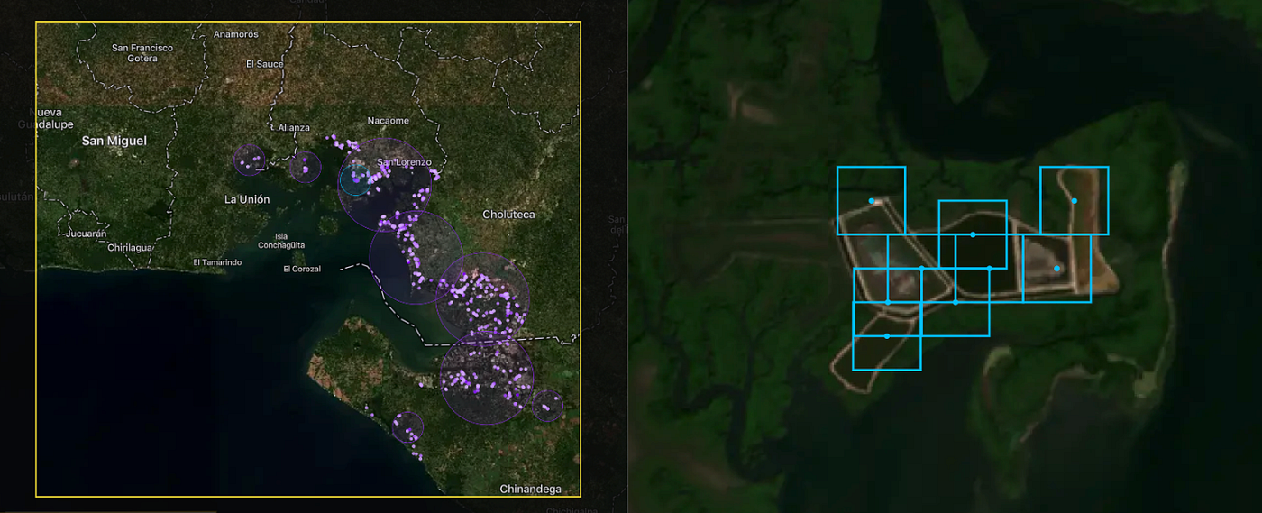
This technological foundation translates directly into powerful tools for understanding and protecting our environment. It empowers journalists (like those at Mongabay and Radio Free Europe), indigenous communities, conservation organizations (like the World Bank), and researchers to uncover hidden environmental changes, monitor industrial footprints, and gather evidence for conservation efforts with unprecedented ease and speed. The figure shows the shrimp farms in the Gulf of Fonseca.
Here are some examples of how Earth Index is being used:
-
Combating Deforestation and Illegal Activities: In collaboration with Mongabay, Earth Index was used to pierce through dense canopy cover and identify hidden, illegal narcotrafficking airstrips in the Amazon. Similarly, the platform can rapidly locate illegal gold mining scars, like those devastating parts of the Yanomami Indigenous Territory, helping to quantify the scale of the problem and guide enforcement efforts.
-
Monitoring Resource Extraction: Radio Free Europe utilized Earth Index to identify over 1300 quarries across the Balkans, revealing that roughly half lacked proper permits, highlighting potential environmental damage and unregulated extraction. This approach can monitor fracking wellpads, rubber processing plants, or other industrial facilities.
-
Protecting Water Quality and Ecosystems: Earth Index can locate Concentrated Animal Feeding Operations (CAFOs) near sensitive waterways to assess runoff risks or identify expansions of shrimp farming into vital mangrove ecosystems.
-
Tracking Agricultural Expansion: The tool helps monitor the conversion of natural habitats into agricultural land by searching for patterns associated with new clearings or specific crop types.
The Infrastructure Challenge: Searching Billions of Vectors Affordably
Generating 3.2 billion high-dimensional vectors is one challenge; hosting and searching them efficiently presents another significant hurdle. Earth Index needed a solution that could:
-
Handle Massive Scales: Searching billions of vectors requires specialized indexing and querying capabilities.
-
Integrate Seamlessly with Geospatial Data: Earth Index heavily relies on geospatial operations (like filtering results within specific administrative boundaries or proximity to rivers). This made PostgreSQL with PostGIS a natural and essential choice for their core database. Standalone vector databases often lack the rich geospatial features required.
-
Maintain Performance: Users need results relatively quickly for the platform to be effective for investigation and monitoring.
-
Control Costs: Storing and searching billions of vectors, especially if requiring vast amounts of RAM for purely in-memory indexes, can become prohibitively expensive for many organizations, particularly non-profits.
Earth Index needed a vector search solution that lived within their chosen PostgreSQL environment, could scale massively, perform well, and wouldn’t break the bank on hardware costs.
Why PostgreSQL Rocks for Planetary-Scale Vectors
While specialized vector databases exist, Earth Index faced a critical need: seamlessly integrating vector similarity search with rich geospatial data and operations. This is where PostgreSQL, combined with extensions, truly shines:
-
Unified Data Platform: PostgreSQL, especially with the powerful PostGIS extension, allowed Earth Index to keep their vector embeddings alongside their crucial geospatial metadata (tile locations, administrative boundaries, proximity to features like rivers). This avoids the complexity and potential synchronization issues of managing separate databases for vector search and relational/geospatial data.
-
Leveraging the Power of SQL & PostGIS: Earth Index could combine vector similarity searches with standard SQL filters and complex PostGIS spatial queries (e.g., “find vectors similar to this example within this specific national park boundary” or “near this river system”) all within a single query interface. Standalone vector databases often lack this mature geospatial query capability.
-
Maturity and Ecosystem: Building on PostgreSQL means inheriting its decades of development, renowned stability, robust tooling, and wide community support – essential for a mission-critical platform like Earth Index.
However, searching 3.2 billion vectors efficiently requires more than just standard PostgreSQL capabilities.
Why Earth Index Chose VectorChord for Performance and Affordability
While the PostgreSQL ecosystem provided the ideal foundation, achieving the required performance and affordability at the scale of 3.2 billion vectors presented a significant challenge. Earth Index needed a solution that could deliver speed without breaking the bank.
Finding the right balance of performance, cost, and integration was challenging. Hutch Ingold, CTO of Earth Genome, explains their considerations:
When we evaluated solutions for our 3.2 billion vectors – recognizing the rapidly evolving tech landscape – standard pgvector didn’t meet our performance requirements at that scale. Dedicated options like Qdrant posed difficulties: hosted versions were too expensive, and self-hosting clustered deployments on our Kubernetes infrastructure seemed insufficiently mature at the time. We also examined cloud services, such as Google’s Vertex AI Vector Search, but the list price of $237,000 per month for our dataset was simply prohibitive.
This is where VectorChord became the enabling technology:
-
Performance Beyond Vanilla PGVector: VectorChord delivers the necessary speed enhancements – up to 5x faster queries, 16x higher insert throughput, and 16x quicker index building – addressing the performance limitations encountered with standard pgvector at this massive scale.
-
Affordable Scale via Disk-Based Indexing: Critically, VectorChord’s optimized disk-based indexing (leveraging cost-effective SSDs) directly counters the prohibitive costs highlighted by the CTO. It avoids the massive RAM requirements of purely in-memory approaches and the exorbitant monthly fees of managed cloud vector services, making the 3.2 billion vector index financially feasible.
-
Native Integration & Scalability: As a PostgreSQL extension, VectorChord provided these benefits within their chosen database, requiring no infrastructure changes. It’s built to scale efficiently, handling the billions of vectors needed for Earth Index’s global monitoring platform while maintaining interactive performance.
VectorChord provided the crucial combination of high performance, massive scalability, and cost-effectiveness directly within the familiar and powerful PostgreSQL environment that Earth Index needed.
Earth Index: Technical Architecture and Setup
To manage its planetary dataset effectively and affordably, Earth Index built its backend on a cluster of three powerful AWS EC2 i8g.16xlarge instances, powered by the latest Graviton4 ARM processor and Nitro SSD. Each provides 512 GB RAM, 64 vCPUs, and 15 TB of NVMe storage, offering a solid foundation for both computation and disk I/O. This setup, costing around $12,000 per month, delivers massive cost savings compared to the estimated $237,000 monthly fee for a comparable managed cloud vector service, making the project economically viable. These instances run PostgreSQL enhanced with VectorChord and PostGIS, efficiently hosting both the vector data and other application components.

The core data resides in a partitioned table structure across the three nodes. The primary table, globe24, stores each tile’s unique ID, its geographic point geometry (geometry(Point, 4326)), a partition key (partkey), and the crucial 384-dimensional AI-generated embedding stored efficiently as halfvec(384). This sharding distributes the 3.2 billion rows across the cluster, allowing for parallel processing.
A key advantage of this architecture is the ability to perform complex, integrated queries. Earth Index commonly executes SQL statements that seamlessly combine VectorChord’s fast vector search (embedding <=> '{vector}'::vector) with PostGIS geospatial filtering (st_within(geom, '{geom}')) and partition pruning (partkey IN (...)). This allows users to find visually similar locations within specific geographic boundaries efficiently. Even with billions of vectors, this integrated approach yields practical performance, achieving a median query latency (p50) of approximately 761 ms for typical searches returning the top 500 results.
Enabling Environmental Action at Scale
By providing a cost-effective, scalable, and tightly integrated vector search solution within PostgreSQL, VectorChord helps enable Earth Index’s groundbreaking work. It allows them to manage their enormous “Planetary DNA” database affordably, ensuring that this powerful tool for environmental monitoring can reach the organizations and communities who need it most.
Join the Earth Index waitlist today to explore the environmental challenges in your neighborhood, understand your ecological footprint, and be part of a global effort to protect the planet.
We are thrilled to see Earth Index leverage VectorChord to turn satellite data into actionable environmental intelligence. Their success demonstrates the power of combining cutting-edge AI, robust database technology, and efficient vector search to address critical global challenges.
Interested in bringing large-scale vector search to your PostgreSQL database? Learn more about VectorChord or get started today!
%[https://github.com/tensorchord/VectorChord]
1.10 - Vector Search Over PostgreSQL: A Comparative Analysis of Memory and Disk Solutions
Introduction: real-world challenges
Specialized vector databases aren’t always needed. With PostgreSQL extensions like pgvector, pgvectorscale, VectorChord (which evolved from pgvecto.rs)****, you get vector search plus relational power—no extra infrastructure. But adoption isn’t seamless. Here’s what real users say:
The query takes 30 seconds for the first time and 100ms if it’s a repeat query. The problem is very slow IO.
Is it normal to take 3 hours to build the index for 12 million rows with 75 dimension vector?
After 13 hours of building index for 200 million vectors of 75 dimensions each, I have noticed a heavy memory usage at 100GB/124GB at 30% of building index, and server will eventually crash.
We’re hitting some challenges, particularly around need for frequent index updates, throughput constraints, lack of parallel index scans and no built-in quantization.
In this article, we’ll take a deep dive into these questions and help you make informed decisions by understanding not only the “what” but also the “why” behind these tools. Let’s explore how to navigate these complexities and choose the right solution for your needs.
What do we value most in a vector database?
In PostgreSQL,
shared_buffersis a crucial memory area acting as the primary cache for data pages, including table data and indexes. By storing frequently accessed vector index blocks in this memory buffer, PostgreSQL significantly reduces slow disk I/O. When a query needs data, PostgreSQL first checksshared_buffers. If the data is present, it’s retrieved quickly without disk access. If not, the data is fetched from disk and loaded intoshared_buffersfor future queries. To configure this, useALTER SYSTEM SET shared_buffers = 'xGB'in psql and restart the server.
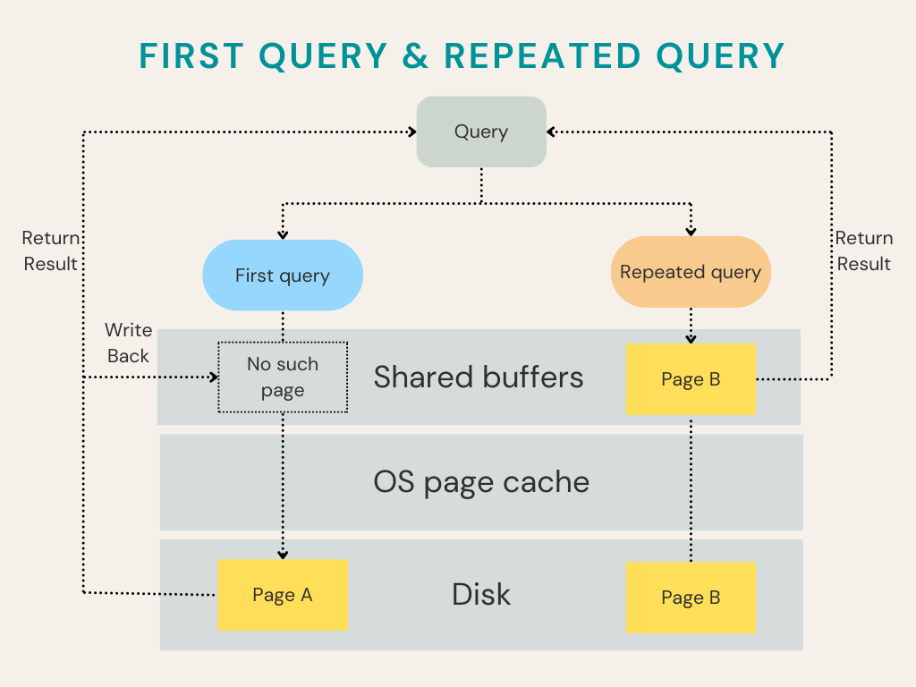
Let’s say you have some vectors in a table, after the index is built, it’s time to start a query. Even though you have set enough shared_buffers for PostgreSQL, it still needs to read the index from disk for the first query. However, for the repeated query, since the vector can be retrieved directly from shared_buffers, it can be much faster.
While the first query after a cold start or index change matters, sustained performance often depends on how quickly queries execute once the ‘hot’ or frequently accessed parts of the index are cached in memory (shared_buffers), mimicking the repeated query scenario. Therefore, optimizing for this cached performance is crucial for many real-world applications.
In this blog, we will compare the performance of vector similarity search extensions in these situations:
-
Query performance when memory is sufficient
-
Query performance when memory is low and disk becomes a bottleneck
We will also discuss other aspects related to index building, such as:
-
Index build speed: How long does it take to build the index? If I have multiple cores in the instance, can it use them all to speed things up? -
Memory usage: How much memory should be reserved for index creation? This is the most important consideration when choosing an instance. -
Disk usage: How many vectors can be hosted on a given amount of disk space? This is also a consideration when choosing an instance that uses non-expandable NVMe SSD (a type of high-performance solid state drive) storage. -
Ease of use: Can I use a simpleCREATE INDEXcommand to create an index? How difficult is it to tune for query performance?
Finally, we will discuss the insertion performance after index building is complete. This is important if the user has streamed data that will trigger frequent index updates.
Experimental setup
Here we present information about the hardware and datasets used in all of the following experiments.
| Vectors in memory | Vectors on disk | Index building | Insertion performance | |
|---|---|---|---|---|
| Instance type | I4I Extra Large |
C6ID Large |
I4I Extra Large |
I4I Extra Large |
| Vcpus | 4 | 2 | 4 | 4 |
| Storage | 937 GB NVMe SSD | 118 GB NVMe SSD | 937 GB NVMe SSD | 937 GB NVMe SSD |
| Memory | 32.0 GiB | 4.0 GiB | 32.0 GiB | 32.0 GiB |
| PostgreSQL shared_buffers | 24.0 GiB | 2.0 GiB | 1.0 GiB | 24.0 GiB |
| Inserted rows | 5,000,000 | 5,000,000 | 5,000,000 | 100 after the index is created |
| Distance metric | L2 distance | L2 distance | / | / |
| Test queries | 10,000 | 10,000 | / | / |
In this table, we show the version of all the extensions we use in these experiments:
| Version | Image | |
|---|---|---|
| VectorChord | v0.2.2 | tensorchord/vchord-postgres:pg17-v0.2.2 |
| pgvector | v0.8.0 | tensorchord/vchord-postgres:pg17-v0.2.2 (with a pgvector v0.8.0 installed) |
| pgvectorscale | v0.6.0 | timescale/timescaledb-ha:pg17.4-ts2.18.2-oss |
Vectors in memory: for small scale data
For a vector search system, if you want the best performance, it’s important to make sure that the entire index is cached in shared_buffers, which is more appropriate on a memory-optimized instance. In this situation, the size of shared_buffers should ideal be large enough to hold the entire index.
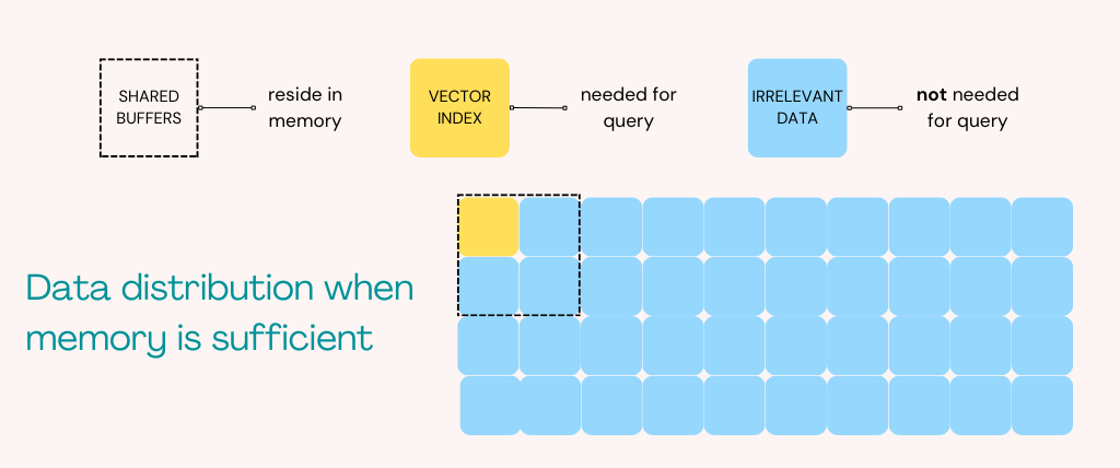
For our experiment, we choose a medium-sized dataset, LAION-5m, which consists of 5 million vectors with 768 dimensions. To host LAION-5m in shared_buffers, we can use the AWS instance I4I Extra Large, with a 937GB NVMe SSD and 32GB of memory.
On this machine, we set the shared_buffers to 24GB and measure the performance of the first query and then the repeated query. The following is the result of the repeated query performance over pgvector, pgvectorscale and VectorChord.
The following graphs illustrate the trade-off between query speed (QPS) and search quality (Recall@10/100). Recall@10 measures the percentage of true nearest neighbors found within the top 10 results. In general, higher QPS can be achieved at the cost of lower recall, and vice versa. A better system may achieve higher recall at the same QPS, or higher QPS at the same recall level. Our goal is typically to maximize QPS while maintaining a high recall target (e.g., 95%).
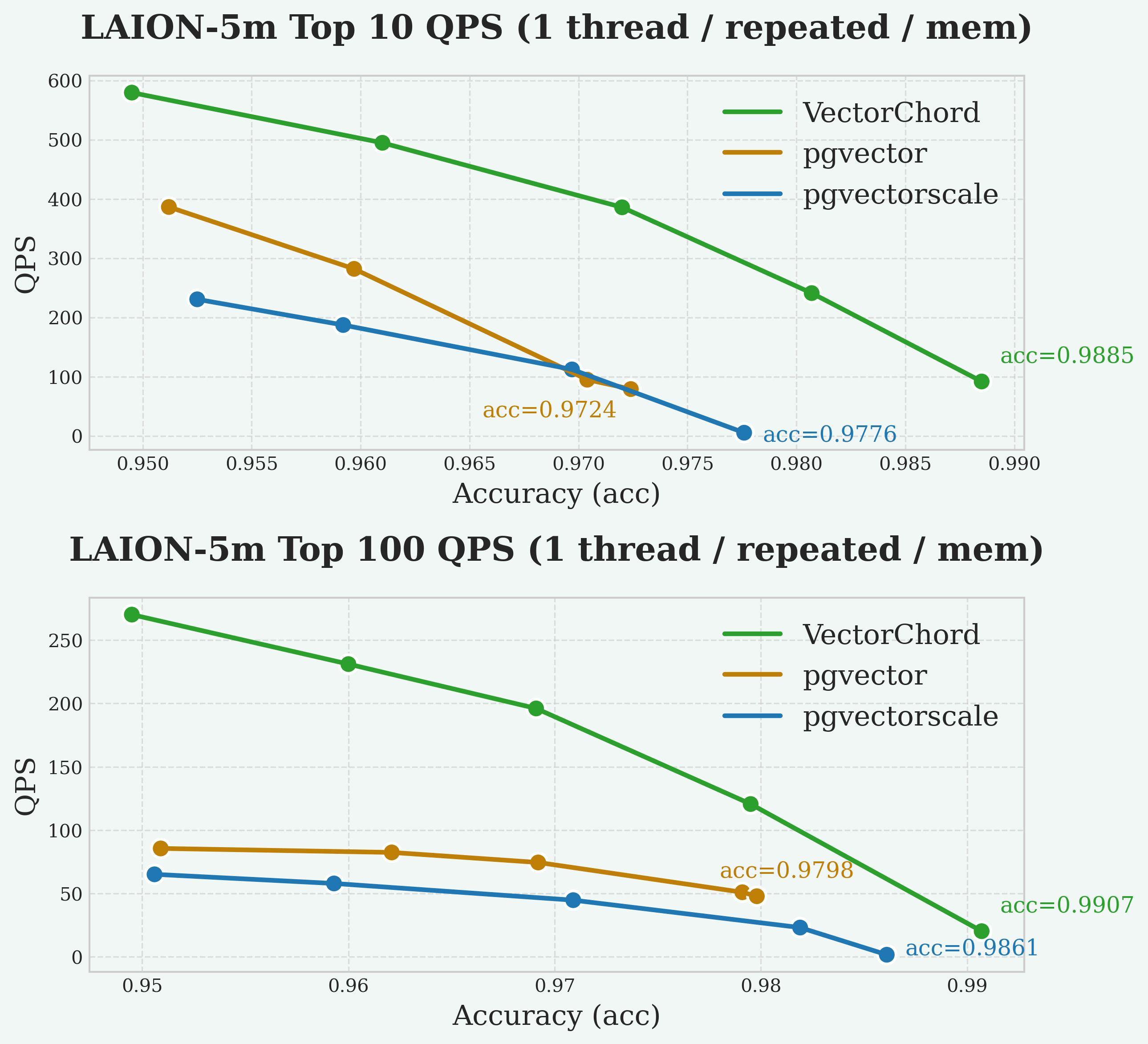
VectorChord’s RabitQ index achieves its speed through optimized vector compression, which allows for faster distance calculations. This compression technique minimizes data movement, resulting in efficient hardware utilization and improved query performance.
To measure first query performance, we cleared shared_buffers before running the 10,000 test queries sequentially. Although the buffer starts empty, index/data pages loaded into the cache by earlier queries within the same test run can sometimes be reused by subsequent queries. This can cause the instantaneous QPS to increase during the run. We report the average QPS across all 10,000 queries to provide a representative measure of performance with a cold cache.
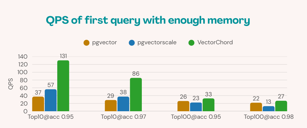
In conclusion, VectorChord consistently achieves higher QPS at high recall levels (e.g., >95% Recall@10) compared to the other extensions. When it comes to the other extensions, pgvectorscale performs better for first query, but once data is cached, pgvector will outperform it.
Vectors in disk: for large scale data
There are times when things are different. For billions of vectors, it is not possible to use memory to store the entire index on a single machine. When the size of the vectors to be read exceeds the size of memory, the speedup effect of shared_buffers is greatly reduced, and most of the data is fetched from disk.
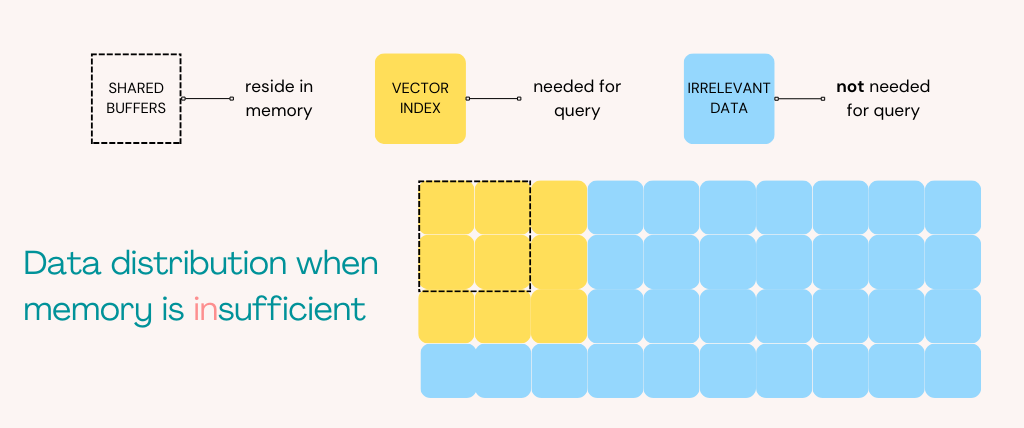
While shared_buffers becomes less effective, the operating system’s page cache can still provide some caching benefits, although its performance is generally lower than shared_buffers.
VectorChord's internal build and pgvectorscale require additional memory to build the index, so it is not possible to build the index on such a small instance with 4GB of memory. To solve this problem, we build the index on another I4I Extra Large instance with 24GB of memory, and then backup and restore the database data directory from AWS S3 for all extensions.
To illustrate this situation, we can host LAION-5m on a much smaller machine, C6ID Large, with 4GB of memory and set shared_buffers to 2GB. This configuration ensures that memory will be insufficient and most queries will be forced to go to disk.
In these cases, the difference in performance between the first and repeated queries will be much smaller due to insufficient memory. Therefore, it’s acceptable to evaluate only the repeated query performance of each extension.
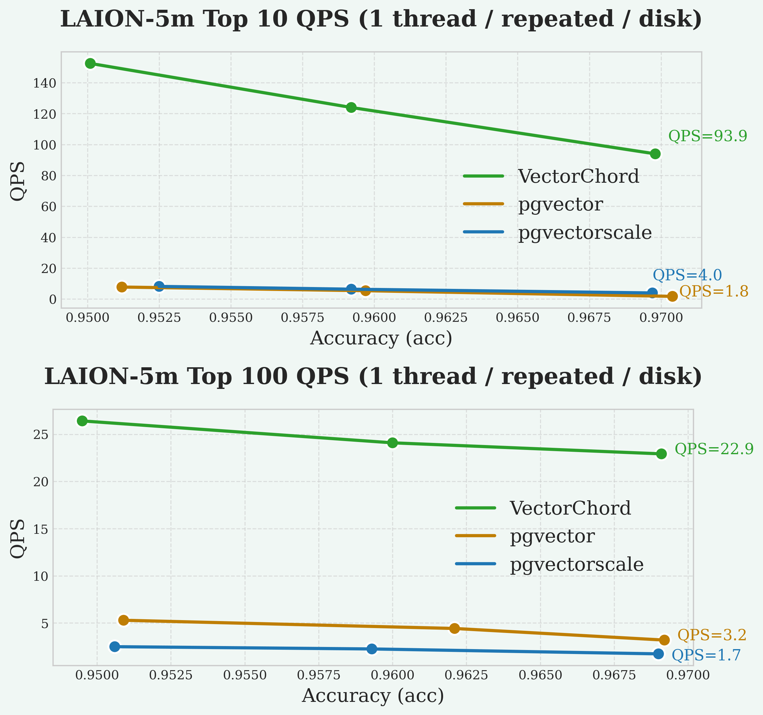
As always, VectorChord consistently achieves higher QPS at high recall levels (e.g., >95% Recall@10) compared to the other extensions, followed by pgvector and pgvectorscale with similar QPS.
Experience in index building
As we discussed earlier, users also care about some index building metrics: Index build time, memory usage, disk usage and usability. We measured these metrics during the CREATE INDEX step of the above experiment on the Laion-5m dataset:
-
Core utilization: Percentage of available CPU cores effectively used during index creation. Higher values indicate better parallelism. -
Index build time: The time taken by the SQL command to build the index. If the index build requires an additional step (VectorChord external build), this should also be included. -
Memory usage: Peak memory usage during the index build, including the 1Gshared_buffersallocated for PostgreSQL. -
Disk usage: The size ofPGDATAon disk after index building is finished, including vectors and the index.
Vectorchord supports two different ways of build indexing, internal build and external build. While internal build is similar to pgvector and pgvectorscale, external build requires an additional k-means clustering. External build usually has better query performance in query and it’s the recommended way for indexing large vectors. If you want to know more about external build in VectorChord, please read our previous blog.
All query performance is measured after an external build, on a standalone machine with A10 GPU. If you insist on using the same I4I Extra Large instance for external builds, the index build time will increase to 50 minutes, which is still competitive.
In this case, we set shared_buffers to 1GB and logged the peak memory usage of each extension. Both VectorChord's internal build and VectorChord's external build are set to 25 iters for K-means clustering. For ease of use, pgvector, pgvectorscale and VectorChord's internal build have similar syntax with a single SQL to build the index, while VectorChord's external build is more complicated.
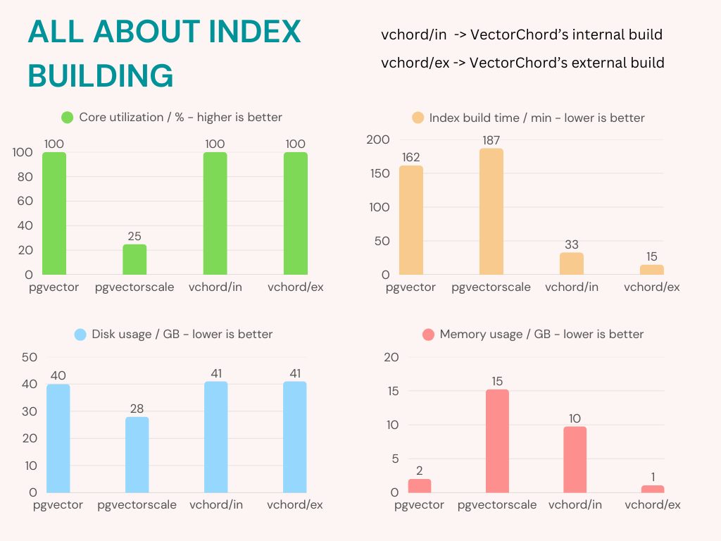
For most aspects, VectorChord's external build gained a leading position, but this partly sacrificed the ease of use, as developers need to implement an additional K-means clustering step outside of PostgreSQL and manage the resulting centroids.
If you want to start with a simple CREATE INDEX command for a straightforward approach, then VectorChord's external build may not be the best choice , you can turn to other extensions / methods:
-
Choose
VectorChord's internal buildfor a faster index build -
Choose
pgvectorif you really don’t have enough memory -
Choose
pgvectorscaleto reduce disk requirements or get better capacity
Insertion performance: for stream-generated data
With streaming vector data, insertion speed can become a new concern. In real-time data analysis systems, the number of new vectors written per second can be very high. Each time new vectors are added to an index, the index itself must be updated. This capability is usually referred to as insertion performance.
For graph-based indexes(pgvector hnsw, pgvectorscale), an index update usually performs multiple searches in the graph and creates new edges for the inserted vector. While clustering-based indexes(VectorChord) just find the right group and add the new vector to it.
So, we set up an experiment to see how well the insertion worked. After building the index for 5 million vectors, we insert another 100,000 random generated vectors into the table one after the other and calculate the insertion time of all.
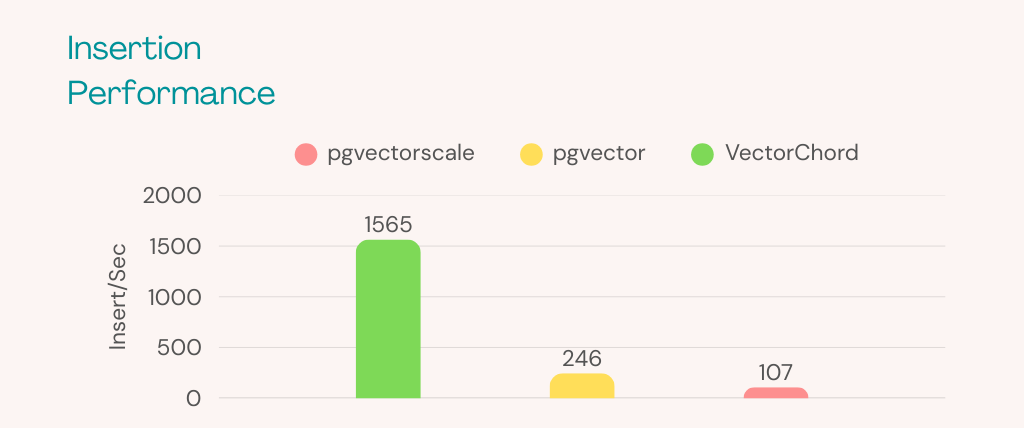
As you can see, VectorChord (1565 Insert/Sec) performs much better than pgvector (246 Insert/Sec) and pgvectorscale (107 Insert/Sec) when inserting data. For most workloads, 100 Insert/Sec is more than enough. However, if you find that a lot of vectors are continuously inserted in your production (for example, 500 Insert/Sec), this could be a problem.
Summary
Based on the results above, this table shows the differences between the three extensions in various aspects. We can see that the main advantage of VectorChord is concentrated in performance, while pgvector and pgvectorscale have their own advantages in terms of usability and capacity.
If you want to see more detailed differences, this table shows them between the three extensions in various aspects. We can see that the main advantage of VectorChord is concentrated in performance, while pgvector and pgvectorscale have their own advantages in terms of usability and capacity.
| pgvector | pgvectorscale | VectorChord | |
|---|---|---|---|
| Ease of use | Easy | Easy, similar to pgvector | Easy (internal), hard (external) with 2-stage build |
| Max dimension can index | 2000 | 16000 | 16000 |
| Ease of tuning | Easy | Moderate, need manually tune query_rescore for different queries | Easy |
| Highest Achievable Recall | Bottom-tier | Mid-tier | Top-tier |
| QPS of repeated query | Mid-tier | Bottom-tier | Top-tier |
| QPS of first query | Mid-tier | Top-tier | Top-tier |
| QPS of disk index | Mid-tier | Mid-tier | Top-tier |
| Speed of index building | Mid-tier, support multiple cores | Bottom-tier, does not support multiple cores | Top-tier, support multiple cores |
| Peak Index Build Memory Usage | 2.1 GB | 15.2 GB | 1.1 GB (external), 9.8 GB (internal) |
| Total Disk Usage | Nearly largest | Smallest | Largest |
Want to know more about how VectorChord compares to other extensions? In future blogs, we will explore the differences of PostgreSQL vector extensions in more scenarios, such as bm25 hybrid search (combining traditional keyword search with vector similarity search) and filtered vector search. Ready to try VectorChord for your vector search needs? Download the extension and feel free to join our Discord community or contact us at support@tensorchord.ai.
%[https://github.com/tensorchord/VectorChord]
1.11 - PostgreSQL Full-Text Search: Fast When Done Right (Debunking the Slow Myth)
You might have come across discussions or blog posts suggesting that PostgreSQL’s built-in full-text search (FTS) struggles with performance compared to dedicated search engines or specialized extensions. A notable recent example comes from Neon’s blog post, “Performance Benchmark: pg_search on Neon” (link).
In their benchmark, Neon compared query performance on their database platform with their pg_search extension (based on Rust’s Tantivy library via pgrx) against the Postgres built-in fulltext search setting with tsvector and GIN index. They commendably stated they optimized this standard setup by adding GIN indexes where appropriate (benchmark code available here).
However, while adding GIN indexes is a necessary first step, their results showing significantly slower performance for the “standard” setup suggest crucial additional optimization steps for PostgreSQL FTS were likely missed. The conclusion that standard FTS is inherently much slower than pg_search might be based on an unintentionally handicapped baseline.
Let’s dive into how to correctly set up and use standard PostgreSQL FTS for optimal performance, addressing the specific configuration flaws likely present in the baseline used in the Neon benchmark, and demonstrating the true speed of built-in FTS. We’ll show concrete numbers demonstrating a ~50x performance increase just by applying these standard optimizations to the baseline configuration.
The Benchmark Setup (Recap from Neon’s Analysis)
The analysis used a table structure similar to this with 10 million log entries:
They tested various query types. Many involved searching the message text field, using queries structured like this in their “standard Postgres” examples:
Even with a GIN index present on message, this query structure and the likely default GIN index settings are where the performance issues for the standard FTS baseline begin.
Our Test Environment Details (Replicating the Baseline Scenario)
To demonstrate the impact of proper optimization on standard FTS, we used the following setup:
-
Instance: AWS EC2
i7ie.xlargewith local NVMe SSD (minimizing I/O impact). -
CPU: 4 vCPUs.
-
PostgreSQL Configuration: PostgreSQL 16 via Docker, configured for the hardware:
-
Parallelism Note: This setup provides
max_parallel_workers_per_gather = 2. The Neon post mentioned their test environment used 8 parallel workers due to larger instances, implying potentially higher parallelism (max_parallel_workers_per_gatherup to 8) than our setup. Our optimized results for standard FTS were achieved with less query parallelism.
Mistake #1: Calculating tsvector On-the-Fly (Major issue)
The sample queries shown in the Neon blog (and common in basic FTS examples) calculate the tsvector within the WHERE clause:
This forces PostgreSQL to:
-
Perform Expensive Computation: Run
to_tsvector()(parsing, stemming, etc.) repeatedly for many rows during query execution. -
Limit Index Efficiency: Prevent the most direct and efficient use of the GIN index, even if one exists on the base
messagecolumn.
The Fix (For a Proper Standard FTS Baseline): Pre-calculate and store the tsvector.
-
Add a
tsvectorcolumn: -
Populate the column:
-
Index the
tsvectorcolumn (withfastupdate=off): (As shown in Fix #1) -
Rewrite queries:
Mistake #2 : Ignoring GIN Index fastupdate (Minor issue)
While Neon’s benchmark correctly identified GIN as the index type for standard FTS, it likely used the default setting: fastupdate=on.
-
fastupdate=on(Default): Prioritizes index update speed by using pending lists. This significantly slows down searches over time, especially on large, static datasets used for benchmarks, as both the main index and growing pending lists must be scanned. It also contributes to index bloat and less efficient page structure. -
fastupdate=off: Prioritizes search speed. Index updates are slower, but the resulting index is more compact and significantly faster to query as there are no pending lists to scan. Essential for read-heavy workloads or benchmarking search performance.
For a fair comparison focused on search speed, the standard FTS baseline should have used fastupdate=off.
The Fix (For a Proper Standard FTS Baseline):
The Performance Impact: A ~50x Speedup for Standard FTS
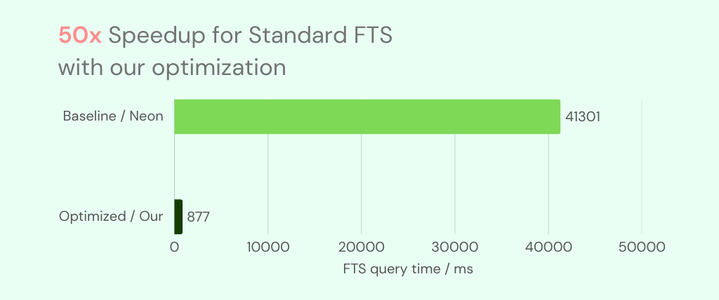
What happens when we apply these standard optimizations to the standard PostgreSQL FTS setup? We tested a query in Neon’s examples on the 10-million-row dataset:
-
Unoptimized Standard FTS (Neon’s Baseline): ~41301 ms (41.3 seconds)
-
Optimized Standard FTS (Our Fixes): ~877 ms (0.88 seconds)
This demonstrates a ~50x speed improvement for standard PostgreSQL FTS achieved simply by applying well-established best practices. This transforms the baseline performance dramatically, suggesting the comparison point used in the Neon benchmark may not have represented the true potential of built-in FTS. This speedup was achieved even with potentially less query parallelism available than in Neon’s tests.
The Grain of Truth: Ranking (ts_rank) Performance
Neon’s analysis did likely highlight a valid point regarding ranking speed. Functions like ts_rank or ts_rank_cd can be relatively slow in standard PostgreSQL compared to just finding matches. This is because ranking requires fetching and processing data for all matching rows before limiting, which can be I/O and CPU intensive.
Beyond Standard FTS: Advanced Ranking with VectorChord-BM25
While standard FTS excels at finding matches quickly, if sophisticated, high-performance ranking is critical, specialized tools are often required. Instead of relying solely on built-in functions, consider VectorChord-BM25.
VectorChord-BM25 is a PostgreSQL extension specifically designed for fast, relevance-based ranking using the well-regarded BM25 algorithm. BM25 goes beyond simple term matching, estimating relevance based on term frequency within a document and inverse document frequency across the entire collection.

Key advantages reported for VectorChord-BM25 include:
-
High Performance: Designed for speed, reportedly outperforming other solutions like Elasticsearch (up to 3x faster) and potentially pg_search for ranking tasks.
-
BM25 Algorithm: Implements a standard, effective relevance ranking model.
-
Specialized Indexing: Uses a dedicated bm25 index type (leveraging optimizations like Block WeakAnd) which is crucial for both performance and calculating the global statistics needed for BM25 scoring.
-
Dedicated Data Type: Introduces a bm25vector type to store tokenized representations suitable for BM25.
If your application heavily relies on the quality and speed of relevance ranking, and standard ts_rank proves insufficient, VectorChord-BM25 presents a powerful, integrated alternative within PostgreSQL.
Conclusion: Standard FTS is Faster Than You Might Think
Standard PostgreSQL FTS is a highly capable and performant feature for finding documents when correctly optimized using tsvector columns and properly configured GIN indexes (with fastupdate=off for reads). Benchmarks suggesting otherwise may be comparing against unoptimized baselines.
For advanced relevance ranking where standard ts_rank falls short, specialized extensions like VectorChord-BM25 offer significant performance improvements by implementing algorithms like BM25 with dedicated data types and optimized indexing strategies.
Choose the right tool for the job: optimize standard FTS first, and if high-performance relevance ranking is paramount, explore dedicated extensions built for that purpose.
%[https://github.com/tensorchord/VectorChord-bm25]
1.12 - VectorChord-BM25: Introducing pg_tokenizer—A Standalone, Multilingual Tokenizer for Advanced Search
We’re excited to announce the release of VectorChord-BM25 version 0.2, our PostgreSQL extension designed to bring advanced BM25-based full-text search ranking capabilities directly into your database!
VectorChord-BM25 allows you to leverage the power of the BM25 algorithm, a standard in information retrieval, without needing external search engines. This release marks a significant step forward, focusing heavily on enhancing the core text processing component: tokenization, unlocking greater flexibility and significantly improved multilingual support.
The Big News: Introducing pg_tokenizer.rs
The cornerstone of VectorChord-BM25 0.2 is a completely refactored and decoupled tokenizer extension: pg_tokenizer.rs.
Why the change? We realized that tokenization – the process of breaking down text into meaningful units (tokens) – is incredibly complex and highly dependent on the specific language and use case. Supporting multiple languages with their unique rules, custom dictionaries, stemming, stop words, and different tokenization strategies within a single monolithic extension was becoming cumbersome.
By moving the tokenizer into its own dedicated project (pg_tokenizer.rs) under the permissive Apache License, we achieve several key benefits:
-
Modularity & Flexibility: Developers can now use or customize the tokenizer independently of the core BM25 ranking logic.
-
Easier Contribution: The focused nature of
pg_tokenizer.rsmakes it simpler for the community to contribute new language support, tokenization techniques, or custom filters. -
Faster Iteration: We can now develop and release improvements to the tokenizer more rapidly without needing a full VectorChord-BM25 release cycle.
-
Enhanced Customization: Users gain significantly more control over how their text, regardless of language, is processed before ranking.
What’s New in Tokenization (Thanks to pg_tokenizer.rs)
This new architecture enables several powerful features in v0.2:
-
Expanded Language Support: Directly handle diverse linguistic needs with dedicated tokenizers like Jieba (Chinese) and Lindera (Japanese), alongside powerful multilingual LLM-based tokenizers (like Gemma2 and LLMLingua2) trained on vast datasets covering a wide array of languages.
-
Richer Tokenization Features: You now have more granular control over the tokenization pipeline:
-
Custom Stop Words: Define your own lists of words to ignore during indexing and search.
-
Custom Stemmers: Apply stemming rules for various supported languages or even define custom ones.
-
Custom Synonyms: Define synonym lists to treat different words as equivalent (e.g., “postgres”, “postgresql”, “pgsql”).
-
Language-Specific Options: Leverage fine-grained controls available within specific tokenizers (like Lindera or Jieba) when needed.
-
Show Me the Code!
Let’s see how easy it is to use the new tokenizer features.
1. Using a Pre-trained Multilingual LLM Tokenizer (LLMLingua2)
LLM-based tokenizers are great for handling text from many different languages.
2. Creating a Custom Tokenizer with Filters (Example: English)
This example defines a custom pipeline, including lowercasing, Unicode normalization, skipping non-alphanumeric tokens, using NLTK English stop words, and the Porter2 stemmer. It then automatically trains a model and sets up a trigger to tokenize text on insert/update.
3. Using Jieba for Chinese Text
(For full examples, including custom stop words and synonyms, please refer to the pg_tokenizer.rs documentation.)
Understanding the Tokenizer Configuration
The new tokenizer system revolves around two core concepts:
-
Text Analyzer: Defines how raw text is processed into a sequence of tokens. It consists of:
-
character_filters: Modify text before splitting (e.g., lowercasing, Unicode normalization). -
pre_tokenizer: Splits the text into initial tokens (e.g., based on Unicode rules, Jieba, Lindera). -
token_filters: Modify or filter tokens after splitting (e.g., stop word removal, stemming, synonym replacement).
-
-
Model: Defines the mapping from the processed tokens to the final integer token IDs used by BM25. Models can be:
-
pre-trained: Use established vocabularies and rules (likebert-base-uncased,llmlingua2). Great for general purpose and multilingual use. -
custom: Build a vocabulary dynamically from your own data, tailored specifically to your corpus and language(s).
-
You can define these components separately or inline them when creating a tokenizer using a simple TOML configuration format passed as a string in SQL.
Get Started with VectorChord-BM25 0.2!
This release significantly boosts the flexibility and power of VectorChord-BM25, especially for users dealing with multiple languages or needing fine-grained control over text processing.
-
GitHub Repository: https://github.com/tensorchord/VectorChord-bm25
-
Tokenizer Documentation: https://vchord.pgsty.com/bm25/tokenizer/
We encourage you to try out version 0.2 and explore the new tokenization capabilities. Your feedback is invaluable – please report any issues or suggest features on our GitHub repository.
Upgrade your PostgreSQL full-text search today with the enhanced multilingual flexibility of VectorChord-BM25 0.2 and pg_tokenizer.rs!
1.13 - Hybrid search with Postgres Native BM25 and VectorChord
In the era of RAG (Retrieval-Augmented Generation), efficiently retrieving relevant data from vast datasets is crucial for businesses and developers. Traditional keyword-based retrieval methods, such as those utilizing BM25 as a scoring mechanism, excel in ranking documents based on term frequency and exact keyword matches. This makes them highly effective for structured queries and keyword-heavy content. However, they struggle with understanding synonyms, contextual nuances, and semantic intent. Conversely, vector-based retrieval captures deep semantic meaning, enabling better generalization across varied queries but sometimes sacrificing precision in exact keyword matches. Hybrid Search bridges this gap by combining BM25’s precision with vector search’s contextual understanding, delivering faster, more accurate, and semantically aware results.
This article explores how to implement Hybrid Search in Postgres using VectorChord-bm25 for keyword-based retrieval and VectorChord for semantic search. By leveraging VectorChord-bm25’s BM25 ranking with the Block-WeakAnd algorithm and VectorChord’s advanced vector similarity capabilities, you can build a robust search system that seamlessly integrates keyword precision with semantic understanding. Whether you’re building a recommendation engine, a document retrieval system, or an enterprise search solution, this guide will walk you through the steps to unlock the full potential of hybrid search.
All related benchmark codes can be found here.
Hybrid Search Explained

Hybrid Search merges the results from vector search and keyword search. Vector search is based on the semantic similarity between the query and the documents, while keyword search relies on the BM25 ranking algorithm. However, it is important to note that BM25 itself is only responsible for scoring documents, while the broader keyword search process also includes steps such as tokenization, indexing, and query parsing. Hybrid Search utilizes reranker or fuses the results from both methods. Fuses include RRF (Reciprocal Rank Fusion) or weighted scoring for multiple recall strategies. Model-based rerank includes cross encoder models like bge-reranker-v2-m3 and multi-vector representation model ColBERT.
%[https://github.com/tensorchord/VectorChord]
What is the VectorChord?
You may be familiar with pgvector, an open-source vector similarity search extension for Postgres. However, scalable or performance-critical scenarios may require a more advanced vector search solution. VectorChord is an excellent choice.
Check out the blog post “VectorChord: Store 400k Vectors for $1 in PostgreSQL” to learn more about its motivation and design.
%[https://github.com/tensorchord/VectorChord-bm25]
What is VectorChord-BM25
VectorChord-BM25 is a PostgreSQL extension for keyword search. It not only implements BM25 ranking but also includes a tokenizer and a Block-WeakAnd index to improve speed.
What is BM25?
BM25 (Best Matching 25) is a probabilistic ranking function used in information retrieval to assess how well a document matches a query. It calculates relevance scores based on term frequency (TF) and inverse document frequency (IDF), while also applying document length normalization. The formula ensures that terms appearing frequently within a document (TF) and those rare across the corpus (IDF) are appropriately weighted, improving search accuracy and relevance. IDF measures how often a word appears across the document collection. The fewer the occurrences, the higher its value. TF represents the frequency of a specific word from the query appearing in the given document. A higher TF indicates a stronger relevance between the query and the document.
Why a Postgres native BM25 Ranking implementation is needed?
In our previous blog post, VectorChord-BM25: Revolutionizing PostgreSQL Search with BM25 Ranking — 3x Faster Than Elasticsearch, my colleague Allen has already provided a detailed and sufficient explanation, which can be referred to.
Tutorial: Use VectorChord-BM25 and VectorChord implement Hybrid Search

In this tutorial, we will guide you through the steps to implement Hybrid Search using VectorChord-BM25 and VectorChord in PostgreSQL. We will cover the following topics:
-
Semantic Search with VectorChord
-
Keyword Search with VectorChord-BM25
-
Rerank
Prerequisites
- Postgres with VectorChord-BM25 and VectorChord
If you want to reproduce the tutorial quickly, you can use the tensorchord/vchord-suite image to run multiple extensions that TensorChord provides.
You can run the following command to build and start Postgres with VectorChord-BM25 and VectorChord.
- Prepare the Embedding Model and Data
For embedding, we can use a pre-trained embedding model like BGE-M3 to generate embeddings for the documents. BGE-M3 is a high-quality embedding model known for its versatility in multi-functionality, multi-linguality, and multi-granularity.
For validation, we use the BEIR dataset, a heterogeneous benchmark for information retrieval. It is easy to use and allows you to evaluate your models across 15+ diverse IR datasets.
First, you need to load your data into PostgreSQL.Then you can use the following SQL query to generate embeddings for the documents.
For embedding:
The data process and embedding generation code can be found here.
Semantic Search with VectorChord
For semantic search, we utilize the RabitQ algorithm, which is highly optimized in the VectorChord PostgreSQL extension. RabitQ is a quantization algorithm for high-dimensional spaces, designed to improve the storage and retrieval efficiency of high-dimensional data, such as embedded vectors.
It achieves this by mapping high-dimensional vectors to a low-dimensional discrete space while preserving the similarity information of the original vectors. This process reduces storage requirements and computational costs while maintaining high retrieval accuracy.
If you find that building the index on your own dataset is too slow, you can utilize external build to accelerate the process. For more details, please refer to our previous blog: Benefits and Steps of External Centroids Building in VectorChord.
Once the index is built, you can use the following SQL query to search for similar documents:
Key-Word Search with VectorChord-BM25
For keyword search, we need to use a tokenizer to convert the text into a BM25 vector, which is similar to a sparse vector that stores the vocabulary ID and frequency.
Let me explain this operation in detail. The tokenize function is used to tokenize the text with the specified tokenizer. In this case, we used the Unicode tokenizer. The output of the tokenize function is a BM25 vector, which is a sparse vector that stores the vocabulary ID and frequency of each word in the text. For example, 1035:7 means the word with vocabulary ID 1035 appears 7 times in the text.
After creating the index, you can calculate the BM25 score between the query and the vectors. Note that the BM25 score is negative, meaning that the higher the score, the more relevant the document is. We intentionally make it negative so that you can use the default ORDER BY to retrieve the most relevant documents first.
Rerank/Fuse
Once you obtain the results from both semantic search and keyword search, you can use a fuse or rerank process to merge the results.
- Fuse (Reciprocal Rank Fusion (RRF))
The advantage of RRF lies in its independence from specific score units; it is based on ranking for fusion, making it suitable for sorting systems with different scoring criteria.
Among them:
-
dis the document. -
nis the number of ranking systems. -
rankis the ranking in the sorting system. -
kis the adjustment parameter, the value is usually 60 (empirical value), used to control the impact of ranking on scores.
- Cross-Encoder model Rerank

In semantic search, we already use Bi-Encoder vectorized the documents and queries separately. But this independent encoding leads to a lack of interaction between the query and the document. Cross-Encoder model will input the query and document as a whole into the model, the model will see the content of both at the same time, capturing the fine-grained semantic relationship between them through the Transformer layer. Compared with RRF, Cross-Encoder model can capture the fine-grained semantic relationship between the query and the document, and it can be more accurate but slower.
Evaluation
We have tested the NDCG@10 with those methods on several BEIR datasets. Here are the top10 results:
| Dataset | Semantic Search | BM25 | Cross-Encoder Rerank | RRF |
|---|---|---|---|---|
| FiQA-2018 | 0.40343 | 0.25301 | 0.42706 | 0.37632 |
| Quora | 0.88433 | 0.78687 | 0.89069 | 0.87014 |
| SCIDOCS | 0.16055 | 0.15584 | 0.17942 | 0.17299 |
| SciFact | 0.57631 | 0.68495 | 0.74635 | 0.67855 |
The table above demonstrates several conclusions:
-
Compared to BM25 and semantic search, the cross-encoder model rerank can significantly improve search performance across different datasets.
-
On some datasets, RRF may lead the performance decrease. Please conduct verification tests before deciding whether to use RRF. If effective, choosing RRF will be a very economical choice, as it is much, much faster than reranking with the cross-encoder model, and almost no resource consumption.
All related benchmark codes can be found here. If you have any questions, please feel free to contact us on Discord or email us at vectorchord-inquiry@tensorchord.ai.
Future Work
The results highlight the great potential of the hybrid search method. In the future, we will focus on the following aspects to advance RAG:
-
Improve the reranking method: Explore the other model-based rerank, such as ColBERT or ColPali, to enhance reranking performance.
-
Integrate graph search: Investigate the use of the Apache AGE extension for graph search and integrate it with the hybrid search method to further improve search performance.
References
1.14 - Vector Search at 10,000 QPS in PostgreSQL with VectorChord
VectorChord is a PostgreSQL extension designed for scalable, high-performance, and disk-efficient vector similarity search, and serves as the successor to pgvecto.rs. In our previous blog post, we showed that with just $250 per month, VectorChord achieved 131 QPS with 0.95 precision on 100 million vectors—demonstrating impressive cost-effective performance for large-scale vector search.

Building on that success, this post focuses on high performance by exploring how VectorChord can reach 10,000 QPS in PostgreSQL. We’ll walk you through how PostgreSQL’s reliable relational foundation integrates with advanced vector indexing to deliver fast, scalable search capabilities, and provide a production-ready setup along with a detailed architecture guide for managing large-scale vector computations even under heavy loads.
Background
High queries per second (QPS) vector search is essential for real-time applications such as recommendation engines, image recognition, and natural language processing. These applications demand rapid, efficient searches to deliver immediate results, which is critical for maintaining user engagement and operational effectiveness. By leveraging PostgreSQL for vector search, you not only benefit from its mature, robust relational capabilities and advanced indexing but also avoid the overhead of managing a separate, specialized vector database. This unified approach simplifies integration and reduces system complexity while still meeting the performance needs of modern applications.
In our experiments, we evaluated performance on LAION datasets of 5 million and 100 million vectors, targeting a 90% precision level to reflect real-world scenarios. We also explored scaling the system with multiple replicas to boost QPS, demonstrating how PostgreSQL can effectively handle demanding vector search workloads while maintaining high performance.
Architecture
Using VectorChord on a multi-node cluster is more difficult than on a single machine. As with other services, a reliable distributed vector search usually has the following requirements:
-
Usability: Declarative configuration management
-
Elasticity: Automatic scaling for nodes based on QPS requirements
-
Load Balancing: Requests are handled effectively across different replica instances
-
High Availability: Having multiple copies of the database and automatically recovering from a replica in case of failure
-
Durability: Secure, persistent storage to ensure data integrity and prevent loss in the event of failures
Therefore, we deploy VectorChord services on AWS EKS with OpenTofu and CloudNativePG to manage the infrastructure that provides the above capabilities. Here are some modules to build the example clusters:
-
OpenTofu: Open source alternative of terraform, used for infrastructure as code (IaC) on AWS EKS
-
CloudNativePG: Manage the full lifecycle of a highly available PostgreSQL database cluster with a primary/standby architecture
-
PGBouncer: Lightweight connection pooler for PostgreSQL, provided by module Pooler of CloudNativePG

Similar to DiskANN, VectorChord can fully utilize disk resources and still maintain competitive performance when memory is insufficient. Besides, VectorChord can also cache indexes in memory to achieve higher query performance.
For more on the technical details of VectorChord, please see our previous post.
To reach the QPS limit, we should assume that the memory can fully hold the dataset and select the AWS machine type based on this standard.
In the following table, we provide the appropriate machine which can hold everything in memory for different sizes of datasets:
| dataset | dim / size | machine / memory |
|---|---|---|
| LAION-5m | 768 / 5,000,000 | r7i.xlarge / 32GB |
| LAION-100m | 768 / 100,000,000 | r7i.16xlarge / 512GB |
Results
As outlined in our documentation, VectorChord accepts two key parameters: nprob and epsilon. Here, nprob defines the number of candidate vectors to scan during a query, while epsilon serves as the threshold for determining whether to rerank results. Both parameters play a critical role in influencing both QPS and recall, allowing users to fine-tune the balance between search speed and accuracy.
-
Lower
nprobwill result in higher QPS and lower recall. -
Lower
epsilonwill result in higher but more unstable QPS and lower recall.
If these parameters are fixed, the precision of each experiment will remain consistent. However, the QPS will still vary depending on the CPU and I/O performance of the underlying hardware. To ensure the precision stays above 0.9, we configured the parameters based on earlier experiments conducted with smaller datasets.
| dataset | nprob / epsilon | recall |
|---|---|---|
| LAION-5m | 20 / 1.0 | 0.9324 |
| LAION-100m | 20 / 1.0 | 0.9042 |
We deployed an r7i.4xlarge instance as the client within the same Availability Zone to query the VectorChord clusters. The clusters were tested with multiple workers ranging from 16 to 128, simulating the concurrency levels typically applied to the database in real-world scenarios. This setup allows us to evaluate how VectorChord performs under varying workloads and concurrency conditions.
With 16 vCPUs, r7i.4xlarge can effectively reduce CPU contention from the client side when the concurrency requests reach up to 128.
In line with common pgbouncer practices, we employed two types of instances: a primary instance for data ingestion and multiple replica instances for read-only workloads. Pgbouncer served as the load balancer, efficiently distributing queries across these backend instances. For the benchmark, we directed our query endpoint to the read-only (ro) pooler, while the read-write (rw) primary instance remained idle during the test. This setup ensures optimal resource utilization and scalability for read-heavy workloads.
For the 5 million dataset, we scaled the number of instances from 5 to 15 to achieve 10,000 QPS. In contrast, for the 100 million dataset, only 2 instances were sufficient to meet the performance standard. The results of these experiments are illustrated in the accompanying figure, demonstrating the scalability and efficiency of VectorChord across different dataset sizes.

Cost
In summary, this is the minimum hardware cost if you need 10000 QPS on such datasets:
| dataset | minimal hardware for 10000+ QPS | number of vcpu | estimate cost per month |
|---|---|---|---|
| LAION-5m | r7i.xlarge × 7 | 4 × 7 = 28 vcpu | $0.2646 × 7 × 720 = $1334 |
| LAION-100m | r7i.16xlarge × 2 | 64 × 2 = 128 vcpu | $4.2336 × 2 × 720 = $6096 |
The cost of the primary instance is excluded from this calculation, as it can be shared and utilized with other PostgreSQL connection poolers, further optimizing resource allocation and reducing overall expenses.
This experiment empowers you to design and scale your own cluster to achieve the ideal level of VectorChord search performance, whether in the public cloud or a private data center. Even in scenarios where performance is the top priority, VectorChord delivers exceptionally competitive pricing, making it a cost-effective solution for high-performance vector search needs.
Summary
Whether you’re launching a startup on a budget-friendly VPS or scaling a large cluster for uncompromised performance, VectorChord opens up unlimited possibilities. While 10,000 QPS is the focus of this post, it’s far from the limit of what VectorChord can achieve.
With its powerful indexing algorithm, VectorChord not only surpasses standard PostgreSQL solutions like pgvector by efficiently utilizing memory and high-speed SSDs, but also outperforms specialized vector databases in handling massive data volumes and high QPS demands. At the same cost, it delivers superior performance while eliminating the complexity of maintaining a separate vector search system.
If you’re eager to explore large-scale vector search solutions, join our Discord community or reach out to us at support@tensorchord.ai. Let’s unlock the full potential of your data together!
%[https://github.com/tensorchord/VectorChord]
1.15 - VectorChord-BM25: Revolutionize PostgreSQL Search with BM25 Ranking — 3x Faster Than ElasticSearch
We’re excited to share something special with you: VectorChord-BM25, a new extension designed to make PostgreSQL’s full-text search even better. Whether you’re building a small app or managing a large-scale system, this tool brings advanced BM25 scoring and ranking right into PostgreSQL, making your searches smarter and faster.
What’s New?
-
BM25 Scoring & Ranking: Get more precise and relevant search results with BM25, helping you find what matters most.
-
Optimized Indexing: Thanks to the Block WeakAnd algorithm, searches are quicker and more efficient, even with large datasets.
-
Enhanced Tokenization: Improved stemming and stop word handling mean better accuracy and smoother performance.
We built VectorChord-BM25 to be simple, powerful, and fully integrated with PostgreSQL—because we believe great tools should make your life easier, not more complicated. We hope you’ll give it a try and let us know what you think.
%[https://github.com/tensorchord/VectorChord-BM25]
BM25
Before we get to the exciting news, let’s take a quick look at BM25, the algorithm that powers modern search engines. BM25 is a probabilistic ranking function that determines how relevant a document is to a search query.
The BM25 formula might look a bit intimidating at first, but let’s break it down step by step to make it easy to understand. Here’s it:
Term Frequency (TF): The term f(q,D) represents how often the query term q appears in document D. The more a term appears in a document, the higher its relevance score. For example, if “AI” appears 5 times in Document A and 2 times in Document B, Document A gets a higher score for this term.
Inverse Document Frequency (IDF): The term IDF(q) measures how rare or common the term q is across all documents. Rare terms (e.g., “NVIDIA”) are given more weight than common terms (e.g., “revenue”). This ensures that unique terms have a greater impact on the relevance score.
Document Length Normalization: The term ∣D∣ represents the length of document D, while avgdl is the average length of all documents in the collection. This part of the formula adjusts the score to account for document length, ensuring shorter documents aren’t unfairly penalized. For instance, a concise report won’t be overshadowed by a lengthy one that only briefly mentions the query term.
Tuning Parameters: The parameters k1 and b allow the formula to be fine-tuned. k1 controls the extent to which term frequency impacts the score, while b balances the effect of document length normalization. These parameters can be adjusted to optimize results for specific datasets.
Consider searching a database of financial reports for “Tesla stock performance.” A report that mentions “Tesla” ten times will score higher than one that mentions it only twice. However, the term “stock” might appear in many reports, so it’s given less weight than “Tesla,” which is more specific. Furthermore, a short, concise report about Tesla’s stock performance won’t be overshadowed by a lengthy report that only briefly mentions Tesla.
Existing Solution in Postgres
Now that we’ve covered the basics, let’s take a look at the existing solutions for full-text search in PostgreSQL.
PostgreSQL provides built-in support for full-text search through the combination of the tsvector data type and GIN (Generalized Inverted Index) indexes. Here’s how it works: text is first converted into a tsvector, which tokenizes the content into lexemes—standardized word forms that make searching more efficient. A GIN index is then created on the tsvector column, significantly speeding up query performance and enabling fast retrieval of relevant documents, even when dealing with large text fields. This integration of text processing and advanced indexing makes PostgreSQL a powerful and scalable solution for applications that require efficient full-text search.
However, PostgreSQL has a limitation: it lacks modern relevance scoring mechanisms like BM25. Instead, it returns all matching documents and relies on ts_rank to re-rank them, which can be inefficient. This makes it challenging for users to quickly identify the most important results, especially when dealing with large datasets.
Another solution is ParadeDB, which pushes full-text search queries down to Tantivy for results. It supports BM25 scoring and complex query patterns like negative terms, aiming to be a complete replacement for ElasticSearch. However, it uses its own unique syntax for filtering and querying and delegates filtering operations to Tantivy instead of relying on Postgres directly. Its implementation requires several hooks into Postgres’ query planning and storage, potentially leading to compatibility issues.
In contrast, VectorChord-BM25 takes a different approach. It focuses exclusively on bringing BM25 ranking to PostgreSQL in a lightweight and native way. We implemented the BM25 ranking algorithm and the Block WeakAnd technique from scratch, building it as a custom operator and index (similar to pgvector) to accelerate queries. Designed to be intuitive and efficient, VectorChord-BM25 provides a seamless API for enhanced full-text search and ranking, all while staying fully integrated with PostgreSQL’s ecosystem.
VectorChord-BM25
Our implementation introduces a novel approach by developing the BM25 index and search algorithm from the ground up, while seamlessly integrating with PostgreSQL’s existing development interfaces to ensure maximum compatibility.
Inspired by the PISA engine, Tantivy, and Lucene, we incorporated the BlockMax WeakAnd algorithm to facilitate efficient score-based filtering and ranking. Furthermore, we employ bitpacking for ID compression to enhance overall efficiency and re-implemented a user data-based tokenizer to more closely align with ElasticSearch’s performance.
The table below compares the Top1000 Queries Per Second (QPS)—a metric that measures how many queries a system can process per second while retrieving the top 1000 results for each query—between our implementation and ElasticSearch across various datasets from bm25-benchmarks:

On average, our implementation achieves 3 times higher QPS compared to ElasticSearch across the tested datasets, showcasing its efficiency and scalability. However, speed alone isn’t sufficient—we also prioritize accuracy. To ensure relevance, we evaluated NDCG@10 (Normalized Discounted Cumulative Gain at 10), a key metric for assessing ranking quality.
NDCG@10 (Normalized Discounted Cumulative Gain at rank 10) is a metric that assesses the relevance of documents within the top 10 positions of a ranked list. It emphasizes not only the relevance of each document but also its position, ensuring higher-ranked relevant documents contribute more to the overall score.
The table below compares the NDCG@10 scores between VectorChord-BM25 and ElasticSearch across various datasets:

We have dedicated substantial effort to align VectorChord-BM25 with ElasticSearch’s behavior, ensuring a fair and precise comparison. As demonstrated in the table, our implementation achieves NDCG@10 scores that are comparable across most datasets, with certain cases even surpassing ElasticSearch (e.g., trec-covid and scifact).
We’ll share the technical details of our alignment efforts in a later section, including how we addressed tokenization, scoring, and other critical components to achieve these results. Before that, let’s explore how to use VectorChord-BM25 in PostgreSQL.
Quick start
To get started with VectorChord-BM25, we’ve put together a detailed guide in our GitHub README that walks you through the installation and configuration process. Below, you’ll find a complete example showing how to use VectorChord-BM25 for BM25 full-text search in Postgres. Each SQL snippet comes with a clear explanation of what it does and why it’s useful.
The extension consists of three main components:
-
Tokenizer: Converts text into a bm25vector, which is similar to a sparse vector that stores vocabulary IDs and their frequencies.
-
bm25vector: Represents the tokenized text in a format suitable for BM25 scoring.
-
bm25vector Index: Speeds up the search and ranking process, making it more efficient.
If you’d like to tokenize some text, you can use the tokenize function. It takes two arguments: the text you want to tokenize and the name of the tokenizer.
One unique aspect of the BM25 score is that it relies on a global document frequency. This means the score of a word in a document is influenced by how frequently that word appears across all documents in the set. To calculate the BM25 score between a bm25vector and a query, you’ll first need a document set. Once that’s in place, you can use the <&> operator to perform the calculation.
Here is an example step by step. First, create a table and insert some documents:
Then tokenize it
Create the index on the bm25vector column so that we can collect the global document frequency.
Now we can compute the BM25 score between the query and the vectors. It’s worth noting that the BM25 score is negative—this is by design. A higher (less negative) score indicates a more relevant document. We intentionally made the score negative so that you can use the default ORDER BY clause to easily retrieve the most relevant documents first.
Other Tokenizers
In addition to BERT, VectorChord-BM25 also supports Tocken and Unicode Tokenizers. Tocken is a Unicode tokenizer pre-trained on the wiki-103-raw dataset with a minimum frequency (min_freq) of 10. Since it’s a pre-trained tokenizer, you can use it similarly to BERT.
Unicode is a tokenizer that builds a vocabulary list from your data, similar to the standard behavior in Elasticsearch and other full-text search engines. To enable this, you need to create a specific one for your data using create_unicode_tokenizer_and_trigger(vocab_list_name, table_name, source_text_column, tokenized_vec_column).
Please check out the tokenizer documentation if you want to know more about it.
Faster than ElasticSearch (Really?)

To ensure our new plugin provides meaningful and relevant results—not just faster performance—we rigorously evaluated VectorChord-BM25 using bm25-benchmarks. We leveraged the widely recognized BEIR benchmark for information retrieval, focusing on two key metrics: QPS (Queries Per Second) to measure speed and NDCG@10 (Normalized Discounted Cumulative Gain at 10) to assess relevance and ranking accuracy.
In our initial version, we were thrilled to see our system achieve 3-5 times higher QPS compared to ElasticSearch. However, we also noticed that on certain datasets, our NDCG@10 scores were significantly lower than ElasticSearch’s. After a thorough analysis, we realized these gaps weren’t caused by our indexing implementation but rather by differences in tokenization approaches.
To address this, we invested considerable effort to align our tokenization process with ElasticSearch’s, ensuring a more accurate and fair comparison.
Issue 1: Stopword List
A stopword is a common word filtered out during text processing because it adds little meaning—for example, words like “the,” “is,” and “at.”
ElasticSearch defaults to using Lucene’s Standard Tokenizer, which relies on a relatively short stopword list. In contrast, our initial implementation utilized NLTK’s much more comprehensive stopword list. As a result, ElasticSearch’s searches include certain stopwords, leading to longer inverted index lists that require additional scanning time—ultimately impacting performance.
Issue 2: Stemming
A stemmer reduces words to their base form, “running” and “ran” both become “run.”
We initially used the snowball stemmer from the rust-stemmer library to handle word variations, but we observed discrepancies compared to ElasticSearch’s implementation. Upon investigation, we discovered that the rust-stemmer’s version of snowball was outdated. Following the guidelines from the official snowball repository, we regenerated the files using the latest version.
When we aligned both the stopword list and stemmer between our system and ElasticSearch, our performance advantage decreased from 300% to 40%. Even so, on three datasets—nq, fever, and climate-fever—a noticeable performance gap persisted. A deeper comparison revealed a subtle but critical detail: in the bm25-benchmark, ElasticSearch preprocesses data differently from other frameworks, which contributed to the remaining discrepancy.
Issue 3: Data Preprocessing
In the BEIR dataset, each document includes both a title and a text field. While most frameworks concatenate these fields into a single string for indexing, ElasticSearch accepts JSON input and indexes the title and text separately. During querying, ElasticSearch performs a multi_match operation, searching both fields independently and combining their scores (using the higher score plus 0.5 times the lower score). This approach yields significantly better NDCG@10 results but requires searching two separate indexes, which can substantially impact performance.
To ensure a fair comparison, we re-ran our ElasticSearch tests by concatenating the title and text fields. With this adjustment, VectorChord-BM25 was able to match ElasticSearch’s results. Interestingly, ElasticSearch’s QPS (geometric mean) increased from 135 to 341 when using concatenated fields, making it 25% faster than VectorChord-BM25’s 271.91 QPS in Top10 query tests. However, in Top1000 tests, VectorChord-BM25 achieved a QPS of 112 compared to ElasticSearch’s 49—making our implementation 2.26 times faster.
This experience highlights the challenges of conducting fair performance comparisons between different BM25 full-text search implementations. The tokenizer is an exceptionally complex and influential component, and ElasticSearch’s intricate default settings add another layer of complexity to the evaluation process.
Future
We’re still in the early stages of this project, and we’ve already pinpointed several areas for performance optimization. Tokenization is an inherently complex process—even for English, we face numerous decisions and trade-offs. Our next step is to fully decouple the tokenization process, transforming it into an independent and extensible extension. This will enable us to support multiple languages, allow users to customize tokenization for better results, and even incorporate advanced features like synonym handling.
Our ultimate goal is to empower users to perform high-quality, relevance-based full-text searches on PostgreSQL with ease. Combined with VectorChord, we aim to deliver a first-class data infrastructure for RAG (Retrieval-Augmented Generation). After all, choosing PostgreSQL is always a solid decision!
If you have any questions about vector search or full-text search in PostgreSQL, feel free to reach out to us! You can connect with us at:
-
Discord: https://discord.gg/KqswhpVgdU
%[https://github.com/tensorchord/VectorChord-bm25]
More Benchmarks
In addition to the Top1000 benchmarks, we have also conducted extensive evaluations for Top10 results. These benchmarks provide further insights into the performance of our implementation across different datasets. If you’re interested in exploring these results in detail, feel free to refer to the data provided here.


1.16 - Do we really need a specialized vector database? (2023)
Notice: This article, originally published in 2023, discusses the relevance and necessity of specialized vector databases, particularly in relation to Postgres and its capabilities. For further insights and discussions on this topic, please refer to the following link: Do we really need a specialized vector database? | Hacker News.
With the popularity of LLM (Large Language Model), vector databases have also become a hot topic. With just a few lines of simple Python code, a vector database can act as a cheap but highly effective “external brain” for your LLM. But do we really need a specialized vector database?
Why does LLM need vector search?
First, let me briefly introduce why LLM needs to use vector search technology. Vector search is a problem that has been around for a long time. The process of finding the most similar object in a collection given an object is vector search. Text/images, etc. can be converted into a vector representation, and the similarity problem of text/images can be transformed into a vector similarity problem.

In the example above, we convert different words into a three-dimensional vector. Therefore, we can intuitively display the similarity between different words in a 3D space. For example, the similarity between “student” and “school” is higher than the similarity between “student” and “food”.
Returning to LLM, the limitation of the context window length is a major challenge. For instance, ChatGPT 3.5 has a context length limit of 4k tokens. This poses a significant problem for LLM’s context-learning ability and negatively impacts the model’s user experience. However, vector search provides an elegant solution to this problem:
-
Divide the text that exceeds the context length limit into shorter chunks and convert different chunks into vectors (embeddings).
-
Before inputting the prompt to LLM, convert the prompt into a vector (embedding).
-
Search the prompt vector to find the most similar chunk vector.
-
Concatenate the most similar chunk vector with the prompt vector as the input to LLM.
This is like giving LLM an external memory, which allows it to search for the most relevant information from this memory. This memory is the ability brought by vector search. If you want to learn more details, you can read these articles (Article 1 and Article 2), which explain it more clearly.
Why is vector database so popular?
In LLM, the vector database has become an indispensable part, and one of the most important reasons is its ease of use. After being used in conjunction with OpenAI Embedding models (such as text-embedding-ada-002), it only takes about ten lines of code to convert a prompt query into a vector and perform the entire process of vector search.
In LLM, vector search mainly plays a role in recall. Simply put, recall is finding the most similar objects in a candidate set. In LLM, the candidate set is all chunks, and the most similar object is the chunk that is most similar to the prompt. In the reasoning process of LLM, vector search is regarded as the main implementation of recall. It is easy to implement and can use OpenAI Embedding models to solve the most troublesome problem of converting text into vectors. The remaining part is an independent and clean vector search problem, which can be well completed by current vector databases. Therefore, the entire process is particularly smooth.
As the name suggests, vector database is a database specifically designed for the special data type of vectors. The similarity calculation of vectors was originally an O(n^2) complexity problem because it required comparing all vectors in the set pairwise. Therefore, the industry proposed the Approximate Nearest Neighbor (ANN) algorithm. By using the ANN algorithm, the vector index is constructed by pre-calculating in the vector database, using the idea of trading space for time, which greatly speeds up the process of similarity calculation. This is similar to the index in traditional databases.
Therefore, vector databases not only have strong performance but also excellent ease of use, making them a perfect match for LLM! (Really?)
Perhaps a general-purpose database would be better?
We’ve talked about the advantages and benefits of vector databases, but what are their limitations? A blog post by SingleStore provides a good answer to this question:
Vectors and vector search are a data type and query processing approach, not a foundation for a new way of processing data. Using a specialty vector database (SVDB) will lead to the usual problems we see (and solve) again and again with our customers who use multiple specialty systems: redundant data, excessive data movement, lack of agreement on data values among distributed components, extra labor expense for specialized skills, extra licensing costs, limited query language power, programmability and extensibility, limited tool integration, and poor data integrity and availability compared with a true DBMS.
There are two issues that I think are important. The first is the issue of data consistency. During the prototyping phase, vector databases are very suitable, and ease of use is more important than anything else. However, a vector database is an independent system that is completely decoupled from other data storage systems such as TP databases and AP data lakes. Therefore, data needs to be synchronized, streamed, and processed between multiple systems.
Imagine if your data is already stored in an OLTP database such as PostgreSQL. To perform vector search using an independent vector database, you need to first extract the data from the database, then convert each data point into a vector using services such as OpenAI Embedding, and then synchronize it to a dedicated vector database. This adds a lot of complexity. Furthermore, if a user deletes a data point in PostgreSQL but it is not deleted in the vector database, then there will be data inconsistency issues. This issue can be very serious in actual production environments.
On the other hand, if everything is done in a general-purpose database, the user experience may be simpler than with an independent vector database. Vectors are just one data type in a general-purpose database, not an independent system. This way, data consistency is no longer an issue.
The second issue is with query language. The query language of vector databases is typically designed specifically for vector search, so there may be many limitations in other types of queries. For example, in metadata filtering scenarios, users need to filter based on certain metadata fields. The filtering operators supported by some vector databases are limited.
In addition, the supported data types for metadata are also very limited, usually only including String, Number, List of Strings, and Booleans. This is not friendly for complex metadata queries.
If traditional databases can support the vector data type, then the aforementioned issues do not exist. Firstly, data consistency is already taken care of as TP or AP databases are existing infrastructure in production environments. Secondly, the issue of query language no longer exists because vector data type is just one data type in the database, so queries for vector data type can use the native query language of the database, such as SQL.
Detailed explanation
However, it is unfair to only compare the disadvantages of vector databases. There are several counterpoints to consider:
-
Ease of Use: Vector databases are designed with ease of use in mind, and users can easily work with them without worrying about the underlying implementation details. However, integrating them with other data storage systems can be a challenge, as mentioned earlier.
-
Performance: Vector databases have a significant advantage over traditional databases in terms of performance for certain use cases. Their design for vector search allows for fast and efficient similarity searches on large-scale datasets with high-dimensional vectors.
-
Metadata Filtering: While metadata filtering capabilities in vector databases may be limited, they can still meet the needs of most business scenarios. However, for more complex metadata queries, a hybrid approach may be needed, where metadata is stored in a separate database or data lake and linked to the vector data in the vector database.
How can you address these issues? In the following section, I will provide my perspective by answering these questions.
Vector databases are easy to use
While it is true that vector databases are easy to use, this is not unique to them. The ease of use of vector databases is mainly due to their abstraction of a specific domain, which allows them to be specifically designed for the most commonly used machine learning programming language, Python, and optimized for vector search scenarios. However, if traditional databases could also support the vector data type, they could offer similar ease of use.
In addition, traditional databases can provide Python SDKs and other integrated tools to meet the needs of most scenarios, as well as standard SQL interfaces to handle more complex query scenarios. Therefore, it is not necessary to use a vector database solely for its ease of use.
Another advantage of vector databases is their distributed design, which allows them to scale horizontally to meet the data volume and QPS requirements of users. However, traditional databases can also meet these requirements through distributed systems. Nevertheless, the decision to use a distributed system should be based on the actual needs of the data volume and QPS requirements, as well as the associated costs.
In summary, while vector databases have their advantages, traditional databases can also provide similar ease of use and distributed capabilities if they support the vector data type. Therefore, the choice between a vector database and a traditional database should be based on the specific needs of the application and the available resources.
Vector databases have better performance
To investigate the performance of vector databases in LLM scenarios, a naive benchmark of vector retrieval was conducted. The benchmark involved N randomly initialized 256-dimensional vectors, and the query time for the top-5 nearest neighbors was measured for different scales of N. Two different methods were used for the test:
-
Numpy was used to perform real-time calculation, which executed completely accurate, non-precomputed nearest neighbor calculation.
-
Hnswlib was used to precompute approximate nearest neighbors.

The benchmark results show that, at the scale of 1 million vectors, the delay of real-time calculation using Numpy is approximately 50ms. Using this as a benchmark, we can compare the time spent on LLM inference after completing vector search. For instance, the 7B model requires approximately 10 seconds for inference on 300 Chinese characters on an Nvidia A100 (40GB). Therefore, even if the query time for real-time accurate calculation of the similarity of 1 million vectors using Numpy is considered, it only accounts for 0.5% of the total delay in the end-to-end LLM inference. Thus, in terms of delay, the benefits brought by vector databases may be overshadowed by the delay of LLM itself in the current LLM scenario. Therefore, we need to also consider throughput. The throughput of LLM is much lower than that of vector databases. Thus, I do not believe that throughput is the core issue in this scenario.
If performance is not the primary concern, what factors will determine the user’s choice? I think it is the overall ease of use, including ease of use for both usage and operation, consistency, and other solutions to database-related issues. Traditional databases have mature solutions for these problems, while vector databases are still in the early stages of development.
Metadata filtering can still meet the needs of most business scenarios
When considering metadata filtering, it’s important to note that it’s not just a matter of the number of supported operators. Consistency of data is also a crucial factor. Metadata in vectors is essentially data in traditional databases, while vectors themselves are indexes of the data. Therefore, it’s reasonable to consider storing both vectors and metadata in traditional databases.
Traditional databases do have the capability to support vector data types and provide similar ease of use and distributed capabilities as vector databases. Furthermore, traditional databases have mature solutions to ensure data consistency and integrity, such as transaction management and data backup and recovery.
Vectors in traditional databases
Since we see vectors as a new data type in traditional databases, let’s take a look at how to support vector data types in traditional databases, using PostgreSQL as an example. pgvector is an open-source PostgreSQL plugin that supports vector data types. pgvector uses exact calculation by default, but it also supports building an IVFFlat index and precomputing ANN results using the IVFFlat algorithm, sacrificing calculation accuracy for performance.
pgvector has done an excellent job of supporting vectors and is used by products such as supabase. However, the supported index algorithm is limited, with only the simplest IVFFlat algorithm supported, and no quantization or storage optimization is implemented. Moreover, the index algorithm of pgvector is not disk-friendly and is designed for use in memory. Therefore, vector index algorithms designed for disk, such as DiskANN, are also valuable in the traditional database ecosystem.

Extending pgvector can be challenging due to its implementation in the C programming language. Despite being open-source for two years, pgvector currently has only three contributors. While the implementation of pgvector is not particularly complex, it may be worth considering rewriting it in Rust.
Rewriting pgvector in Rust can enable the code to be organized in a more modern and extensible way. Rust’s ecosystem is also very rich, with existing Rust bindings such as faiss-rs.

As a result, pgvecto.rs was created. pgvecto.rs currently supports exact vector query operations and three distance calculation operators. Work is underway to design and implement index support. In addition to IVFFlat, we also hope to support more indexing algorithms such as DiskANN, SPTAG, and ScaNN. We welcome contributions and feedback from the community!
pgvecto.rs offers a modern and extensible codebase with improved performance and concurrency. Its design and implementation allow seamless integration with other machine learning libraries and tools, making it an ideal choice for similarity search scenarios.
With ongoing development, pgvecto.rs aims to be a valuable tool for data scientists and machine learning practitioners. Its support for various indexing algorithms and its ease of use make it a promising candidate for large-scale similarity search applications. We look forward to continuing development and contributions from the community.
Future
As LLMs gradually move into production environments, infrastructure requirements are becoming increasingly demanding. The emergence of vector databases is an important addition to the infrastructure. We do not believe that vector databases will replace traditional databases, but rather that they will each play to their strengths in different scenarios. The emergence of vector databases will also promote traditional databases to support vector data types.
We hope that pgvecto.rs can become an important component of the Postgres ecosystem, providing better vector support for Postgres. Its implementation in Rust and support for various indexing algorithms make it a promising candidate for large-scale similarity search applications. We believe that its development and contributions from the community will help it become a valuable tool for data scientists and machine learning practitioners.
1.17 - Supercharge vector search with ColBERT rerank in PostgreSQL
Traditional vector search methods typically employ sentence embeddings to locate similar content. However, generating sentence embeddings through pooling token embeddings can potentially sacrifice fine-grained details present at the token level. ColBERT overcomes this by representing text as token-level multi-vectors rather than a single, aggregated vector. This approach, leveraging contextual late interaction at the token level, allows ColBERT to retain more nuanced information and improve search accuracy compared to methods relying solely on sentence embeddings.

As illustrated in the above image, ColBERT encodes each document/query into a list of token vectors and computes the MaxSim during the query time.
Token-level late interaction requires more computing power and storage. This makes using ColBERT search in large datasets challenging, especially when low latency is important.
One possible solution is to combine sentence-level vector search with token-level late interaction rerank, which leverages the efficiency of approximate vector search and the high quality of multi-vector similarity search.
The multi-vector approach is not limited to pure text retrieval tasks; it can also be used in visual document understanding. For multimodal retrieval models, state-of-the-art models like ColPali and ColQwen directly encode document images into multi-vectors and demonstrate stronger performance compared to OCR-to-text approaches.
This blog will demonstrate using the PostgreSQL extension VectorChord and pgvector with ColBERT rerank.
Tutorial
Assume we already have the documents, let’s create a table to store all of them:
Here we created a table with sentence-level embedding and token-level embeddings.
There are numerous embedding APIs and open-source models. You can choose the one that fits your use case.
For token-level embedding:
ColBERT model produces 128-dim vectors by default.
To insert the data:
For the vector search part, we can use VectorChord to build a high-performance RaBitQ index:
To speed up the indexing building process, we can utilize the external centroids build. Check “Benefits and Steps of External Centroids Building in VectorChord” for more details.
Now, we can query the PostgreSQL:
To support MaxSim rerank, we’ll need to create a function:
Now, we can rerank the documents retrieved by vector search:
Evaluation
We have tested this method on several BEIR datasets. Here are the results:
| Dataset | Search NDCG@10 | Rerank NDCG@10 |
|---|---|---|
| fiqa | 0.23211 | 0.3033 |
| quora | 0.31599 | 0.3934 |
This shows that ColBERT reranking can significantly enhance the results of vector searches.
All the related benchmark codes can be found here.
Future work
Vector search and full-text search with ColBERT rerank can further improve performance. We’re also working on the PostgreSQL BM25 extensions. Stay tuned.
References
1.18 - ARM + VectorChord: Affordable, Fast Vector Search
ARM64 is quietly becoming a go-to for cost-effective cloud servers, especially on AWS. With ARM-based processors like the Graviton series (Graviton3 and Graviton4), you can save a good chunk of money without sacrificing performance. These ARM64 instances are way more affordable than traditional x86 ones, making them a solid choice for balancing cost and performance in the cloud.
That said, ARM’s architecture differs from x86, so software that isn’t optimized for it might run slower due to emulation. This is where VectorChord steps in—a PostgreSQL extension designed for scalable, high-performance, and disk-efficient vector similarity search. As the successor to pgvecto.rs, VectorChord lets you store a whopping 400,000 vectors for just $1, delivering massive savings: 6x more vectors than Pinecone’s optimized storage and 26x more than pgvector / pgvecto.rs for the same price.
By leveraging platform-specific features like AVX-512 on x86_64 and SVE on ARM64, VectorChord ensures efficient vector search performance across different systems. Whether you’re on ARM64 or x86, VectorChord keeps things running smoothly, making it a reliable and versatile solution for modern computing environments. In short, ARM64 is a great option for saving money, and VectorChord is here to make sure your vector search is fast, efficient, and budget-friendly.
Benchmark Setup
We ran benchmarks on three AWS EC2 instances to evaluate VectorChord’s performance across different setups. Here’s a breakdown of our choices and findings:
| instance | i4i.xlarge | i8g.xlarge | i7ie.xlarge |
|---|---|---|---|
| Memory | 32 GiB | 32 GiB | 32 GiB |
| vCPUs | 4 | 4 | 4 |
| CPU generation | 3rd gen Intel Xeon | AWS Graviton4 | 5th gen Intel Xeon |
| CPU Architecture | x86_64 | arm64 | x86_64 |
| Storage | 937 GB NVME SSD | 937 GB NVME SSD | 2500 GB NVME SSD |
| cost | $0.1158 hourly | $0.1162 hourly | $0.1723 hourly |
The i8g.xlarge (ARM-based) is priced almost identically to the i4i.xlarge but offers a noticeable boost in CPU performance. When compared to the i7ie.xlarge, which has comparable CPU capabilities, the i8g.xlarge comes in at nearly half the cost, making it a much more budget-friendly option.
Test result
To showcase how competitive ARM64 machines are for vector search, we ran the same LAION benchmark test across all selected machine types. We measured key metrics like index construction speed, query throughput (QPS), and recall rates under different search parameters.
This benchmark involves inserting 5 million vectors (each with 768 dimensions) and running 1,000 queries on them. The results below highlight the index build time and query performance for each cluster, giving a clear picture of how ARM64 stacks up against traditional x86 setups.

As the results show, VectorChord running on the i8g.xlarge (ARM64) delivers about a 30% improvement in throughput compared to the i4i.xlarge**,** even though both are priced similarly. On the other hand, the more expensive i7ie.xlarge, which costs 50% more, only offers a modest 15% performance boost over the i8g—far from justifying its higher price tag. Additionally, the index construction time on the ARM-based i8g is significantly faster, which was a surprising and welcome advantage.
In short, the ARM-based i8g.xlarge strikes a better balance between performance and cost when compared to both the i4i.xlarge and i7ie.xlarge. This aligns perfectly with the core value VectorChord brings to its users: more performance for less cost. Whether you’re looking to save money or maximize efficiency, the combination of ARM64 and VectorChord is a clear winner.
1.19 - Why HNSW is Not the Answer
HNSW (Hierarchical Navigable Small World) has become the go-to algorithm for many vector databases. Its multi-layered graph structure and ability to efficiently navigate vector embeddings make it particularly appealing. However, despite its apparent advantages, HNSW may not be the optimal solution for large-scale and dynamic vector similarity search. In this blog post, we challenge the dominance of HNSW and explore why disk-based alternatives, such as IVF (Inverted File Index), might be more practical for massive datasets.
The Appeal of HNSW
HNSW offers several advantages:
-
Efficient Search: Its graph-based structure enables quick nearest-neighbor searches, especially for smaller datasets.
-
Incremental Updates: The ability to add new vectors incrementally without needing to rebuild the index is a major benefit for dynamic environments.
-
High Recall: HNSW delivers high recall with relatively low latency, making it an ideal option for real-time applications.
However, these benefits come with trade-offs that become more noticeable as dataset sizes increase.
The Problem of HNSW
One of the main challenges of HNSW is its significant dependence on memory for indexing and search operations. Here are the primary issues that emerge:
-
Memory Overhead: Traversing HNSW’s graph structure involves highly random access patterns. The entire dataset must be stored in memory to achieve reasonable performance. This becomes infeasible for large-scale datasets with billions of high-dimensional vectors due to exorbitant memory requirements.
-
Performance Sensitivity to Memory Size: HNSW’s performance degrades sharply if the memory is even slightly insufficient to hold all vectors. In such cases, swapping data to disk drastically impacts search speed, making it impractical for systems with constrained memory.
-
Unsuitability for Disk-Based Environments: HNSW is fundamentally designed for in-memory operations and performs poorly in disk-oriented scenarios, such as PostgreSQL. Its reliance on frequent random access patterns makes it incompatible with the sequential access nature of disk storage.
-
Insertion and Deletion Costs: Updating the index in HNSW involves cascading modifications throughout the graph, leading to significant computation and write amplification. This makes insertion and deletion operations both slow and resource-intensive.
In contrast, disk-based solutions like IVF excel in scenarios requiring scalability and efficiency at the cost of minimal complexity.
Why IVF Can Be Faster Than HNSW

A critical observation across all vector search algorithms is that their performance largely hinges on the number of distance computations they perform. Minimizing these computations is essential for improving search speed. Although the original IVF index required scanning 1% to 5% of the total vectors, modern advancements in quantization and optimization have significantly enhanced its efficiency, making IVF a strong competitor to HNSW.
Quantization: The Game Changer
Quantization compresses high-dimensional vectors into compact representations. For instance:
-
RaBitQ: Leverages concentration of measure phenomena to enhance binary and scalar quantization accuracy, quantizing each dimension into 1 bit for a 32x compression ratio.
-
Product Quantization (PQ): Works by dividing the vector space into subspaces, quantizing each subspace independently to minimize approximation error. This method offers flexible compression ratios from 4x to 64x in FAISS, enabling finer compression and faster approximate searches.
-
Scalar Quantization (SQ): Quantizes each vector dimension independently by dividing its range into discrete levels, typically achieving a 4x compression ratio by converting from float to int8.
-
ScaNN: Uses anisotropic vector quantization to optimize inner product accuracy by penalizing errors in directions that impact high inner products, achieving superior recall and speed.
Quantization reduces memory and disk space usage significantly—often by a factor of 32x when converting floats into bits—while drastically lowering computational overhead. Despite some loss of precision, quantization makes vector comparisons far more efficient. For example, by compressing floating-point numbers into bits, this complexity is reduced by a factor of 32. Additionally, binary operations are generally more efficient compared to floating-point operations, further enhancing performance. With fast-scan optimizations, these computations are further accelerated via efficient CPU register lookups. Combined with IVF, many quantization methods consistently outperform HNSW in both speed and scalability. The typical workflow involves:
-
Initial Search: Leveraging compressed representations to rapidly identify candidate vectors.
-
Reranking: Refining results using full-precision distance calculations on a smaller subset of candidates.
Comparing RaBitQ+IVF and HNSW
IVF with quantization provides a highly efficient way to store all quantized vectors in memory. By leveraging RaBitQ, memory usage is reduced by a factor of 32 compared to full-size vectors, allowing the entire quantized dataset to fit in memory. This design enables the index to rapidly retrieve approximate nearest neighbors using bit vectors and rerank them with full-precision vectors fetched from disk. For a typical Top-10 query, IVF fetches only 100-200 vectors from disk, compared to HNSW, which may require 800-1000 vectors. This efficient approach achieves an optimal balance between memory usage and disk access, offering outstanding cost-performance benefits.

While similar quantization techniques could theoretically be applied to HNSW, practical constraints reduce their effectiveness:
-
Vector Packing: Fast scan optimization relies on packing 32 compressed vectors together, which is incompatible with HNSW’s graph structure.
-
Random Access Costs: HNSW involves frequent random access across graph nodes and edges, making traversal inefficient. In contrast, IVF organizes vectors sequentially in posting lists, enabling faster prefetching and efficient sequential scans.
-
Reranking Costs: Both IVF and HNSW share similar reranking computational costs due to their reliance on quantized representations in the first stage.
Ultimately, the performance difference between quantized IVF and HNSW is likely minimal, but IVF stands out with its simplicity and efficiency.
| Feature | IVF | IVF + RaBitQ | HNSW |
|---|---|---|---|
| Indexing Method | KMeans can be offloaded to GPU | KMeans + Quantization | Nearest Neighbor Graph, need to keep everything in memory |
| Overlapped Data Across Query | Centroids | Quantized vectors | No |
| Scalability | Limited by CPU and memory | Outstanding | Limited by memory |
| Insertion/Deletion | Simple (updates posting lists) | Simple (updates posting lists) | Complex (cascading graph changes) |
| Search Speed | Slow | Extremely Fast with Quantization | Fast with sufficient memory |
| Overall Complexity | Low | Low | High |
Operational Simplicity of IVF
IVF’s simplicity makes it a more practical choice for real-world applications:
-
Insertion and Deletion: In HNSW, these operations trigger cascading modifications throughout the graph, resulting in significant computation and write amplification. IVF, in contrast, only requires updating the relevant posting list.
-
Disk-Based Storage: IVF’s reliance on disk-based indexing enables it to scale efficiently without the prohibitive memory costs associated with HNSW.
-
Adaptability: IVF can be easily combined with advanced quantization techniques, enabling further optimizations.
Conclusion
While HNSW has solidified its reputation as a fast and accurate algorithm for vector similarity search, it is not without limitations. Its memory-intensive nature and operational complexity make it less suitable for large-scale applications. In contrast, IVF offers a scalable and cost-effective alternative, particularly when paired with modern quantization techniques.
As the demand for vector search continues to grow, practitioners must carefully evaluate the trade-offs between memory-based and disk-based solutions. HNSW may dominate small to medium-scale applications, but for massive datasets, it’s time to look beyond HNSW and embrace simpler, scalable approaches like IVF.
If you’re interested in such databases, check out VectorChord.
%[https://github.com/tensorchord/VectorChord/]
1.20 - Benefits and Steps of External Centroids Building in VectorChord
Clustering is an important component in vector search, and the k-means algorithm remains one of the most widely used techniques. However, its simplicity comes with a significant drawback: resource-intensive computation can render it impractical for large datasets. This blog explores why this challenge arises and how leveraging external builds to overcome it. We also share insights into our approach to implementing this solution.
Why we need it

VectorChord uses IVF + RaBitQ to perform vector search. The quality of the IVF cluster can heavily affect search precision and speed. K-means usually takes dozens of rounds before convergence. For each round, all the sampled vectors need to be assigned to the nearest cluster. This is the most computationally intensive part. The good news is that this process can be easily parallelized.
However, the vector search instances usually don’t have such kind of resources to perform this parallel computation, doing so can dramatically affect the vector search service. In this case, it’s natural to utilize external instances to accelerate the indexing phrase.
External K-means
The source vectors could be several times larger than the instance memory. To avoid out-of-memory, we can sample the vectors before clustering them. A good choice of cluster number is:
Usually, we need to sample at most 256 * n_cluster vectors. This can be done by reservoir sampling if the data can not fit into the memory.
If you have a ready-to-use GPU environment, it can run tens or even hundreds of times faster than a CPU instance. Otherwise, you may find that half or most of the time is spent on spawning instances, transferring data, and sampling instead of computing.
The following clustering experiments are performed on an H100 SXM5 instance with faiss-gpu (max_iter=25), which costs $3.29 / hr. Comparing to an i4i.8xlarge instance with faiss-cpu (max_iter=25), which cost $2.746 / hr. CPU instances are about 60 times more expensive to cluster than GPU instances.
| Dataset | Cohere (1024 × 10m) | MS MARCO (768 × 100m) |
|---|---|---|
n_cluster |
16384 | 65536 |
| GPU K-means time | 80s | 960s |
| CPU K-means time | 5850s | 68420s |

Stay tuned for our upcoming cloud support of external builds.
It is obvious that a larger n_cluster results in an exponential growth of time. Also, K-means can not maintain a relative balance if the n_cluster is large.

A good way to overcome this is the hierarchical K-means. Usually, 2 layers are enough. We could build a n_cluster = [40, 100] hierarchical K-means instead of n_cluster = 4000. This also trades the heavy computation for IO and light computation, and it’s a good choice when you want to use CPU instances for large datasets.
Steps

Assuming we already have the vectors stored in VectorChord, we will need to:
-
export the vectors and upload them to S3
-
spawn an instance to run the K-means clustering
-
insert the centroids back into the VectorChord
-
build the index with an external centroids table
We provide some scripts to make it easy to get started:
You can clone the repo and try it by yourself:
Summary
In conclusion, leveraging external centroids building in VectorChord offers significant advantages for handling large datasets in vector search. By utilizing external resources for the computationally intensive K-means clustering, we can enhance the efficiency and precision of the search process. This approach not only mitigates the resource constraints of vector search instances but also allows for faster processing times, especially when using GPU environments. Using hierarchical K-means further optimizes the process by balancing computation and I/O operations, making it feasible to use CPU instances for extensive datasets.
1.21 - VectorChord: Store 400k Vectors for $1 in PostgreSQL
We’re pleased to announce our new vector search extension for PostgreSQL, providing a highly cost-effective way to manage large vectors. Using VectorChord, you can achieve a QPS of 131 with 0.95 precision on 100 million 768-dimensional vectors for the top 10 queries. This setup costs only $250 monthly and can be hosted on a single machine.
This means you can store 400k vectors for only $1, allowing you to save significantly: 6x more vectors compared to Pinecone (storage optimized instance) and 26x more than pgvector/pgvecto.rs for the same price.

In the monthly cost comparison for storing vectors, based on MyScale benchmark data, the chart highlights how VectorChord emerges as an affordable option, priced at just $247 for storing 100 million vectors. In contrast, Pinecone, despite its optimized storage, costs $1,600 per month, while Qdrant is priced at $4,374. pgvector/pgvecto.rs has a considerably higher cost of $6,580.

%[https://github.com/tensorchord/VectorChord]
HNSW’s problem
As the successor to pgvecto.rs, VectorChord has gained valuable insights from its predecessor. While many vector databases or extensions (including pgvecto.rs) perform well with datasets of around 1 million, they often struggle when scaling up to larger sizes, such as from 10 million to 100 million. Traditional HNSW-based vector databases face specific challenges with larger datasets:
-
Long index build time: It typically takes over 2 hours to build an index for 5 million records.
-
High memory requirements: Storing a dataset of 10 million vectors can require as much as 40GB of memory.
VectorChord’s solution: Disk-friendly IVF+RabitQ
VectorChord employs IVF (Inverted File Index) along with RaBitQ
quantization to provide fast, scalable, and accurate vector search capabilities. This method compresses 32-bit vectors into compact bit representations, significantly reducing computation demands. Most comparisons are conducted using these compressed vectors, while full-precision calculations are reserved for an adaptive reranking phase applied to a smaller subset, ensuring both speed and recall are preserved.
Many people think that IVF has a less favorable recall/speed tradeoff than HNSW and involves many configurations for optimization. However, it’s a complex issue, and we’ll explain it briefly now, with a detailed post on the topic coming later.
IVF vs HNSW
A significant portion of the time taken by vector search algorithms is dedicated to distance computation. To enhance speed, it’s essential to minimize distance comparisons as much as possible. The original IVF struggles in this area, usually necessitating a scan of 1% to 5% of the total vectors, which is considerably higher than what HNSW requires.
However, RabitQ presents an innovative approach that allows for the compression of a 32-bit vector into just 1 bit. While this compression results in some loss of precision, it greatly reduces computational requirements. With the fast scan optimization, we can achieve calculations that are over 100 times faster than traditional vector distance computations.
You might wonder about the recall. We can rerank additional vectors to enhance the recall rate, and full precision distance computation is only necessary during the reranking phase. RaBitQ guarantees a sharp theoretical error bound and provides good empirical accuracy at the same time. This is why IVF can be faster than HNSW.
Here are some initial benchmark results for the GIST dataset, which consists of 1 million vectors in 960 dimensions. With equivalent recall, VectorChord’s QPS could be twice that of pgvector. More details will be provided in the Benchmark section.

External Index build
The original IVF method typically needs to scan 1–5% of the dataset, which can be slow. By using RaBitQ and fast scan optimization, VectorChord aims to speed up calculations by cutting down the number of full precision vectors that need to be fully compared. This approach helps create a stable and scalable vector search system that works well with the PostgreSQL storage system. As a result, users can use physical replication and other PostgreSQL features along with VectorChord.
Built on IVF, VectorChord allows KMeans clustering to be conducted externally (such, as on a GPU) and easily imported into the database. We performed tests to measure indexing and insert time on an AWS i4i.large instance, which has 2 vCPUs, and 16 GB of RAM. The dataset used for this test was GIST 1M. We inserted 700,000 vectors, built the index, and then added another 300,000 vectors. After warming up the system, we performed queries using a single thread. During this process, we evaluated both the index build time and the insert time. Here are the results:

VectorChord takes 186 seconds to build the index by utilizing a separate machine for KMeans clustering, making it 16 times faster than pgvector. Additionally, the insert time is also 14 times faster than that of pgvector. As we know, indexing is the most resource-intensive part of vector databases, requiring significant computation and increasing the demand for CPUs and memory. By utilizing a more capable machine to build the index and then importing it to a smaller machine for querying, it becomes possible to support billions of vectors on a single machine.
Benchmark
We conducted additional experiments to assess performance and costs more thoroughly using the LAION 5M and 100M datasets.
LAION 5M
We had an experiment using the LAION 5M dataset, and the results were encouraging for Vectorchord. It consistently achieved higher queries per second (RPS) compared to other platforms. While many databases struggle to maintain a balance between speed and accuracy as recall increases, Vectorchord managed to remain efficient even at higher recall levels. This characteristic could make it a suitable option for applications needing both quick responses and precision.

The experiment utilizes the Myscale single thread benchmark, and we conducted it on an r6a.xlarge machine, which features 4 vCPUs, 32GB of memory, and 200GB of EBS storage. The parameters set for the experiment include an nlist of 8192, a shared buffer of 28GB, JIT disabled, and an effective I/O concurrency of 200. We ran the experiment twice without prewarming.

The machine we used, an r6a.xlarge, costs around $165.56 per month, while the Zilliz Performance 4CU is priced at approximately $460 per month. Notably, we achieved comparable performance in the Top 100 on the LAION 5M dataset.
LAION 100M, on a single machine
Furthermore, due to its disk-friendly indexing, increasing a single machine’s disk capacity can proportionally enhance the maximum number of vectors VectorChord can hold, potentially allowing for storage of 1 billion or more.
To assess scalability, we performed experiments on the LAION 100M dataset (768 dimensions) using an AWS i4i.xlarge instance, which is an economical configuration priced at $250 per month.

It features just 4 CPUs and 32 GB of memory, with 937 GB of SSD used to store the 100 million vectors. In this setup, we achieved a QPS of 16.2 @ recall 0.95 for the top 10 results and 4.3 @ recall 0.95 for the top 100 results with a single-thread query. Here are the impressive results:

While maintaining a recall greater than 0.95, we also assessed the multi-thread QPS on this 4-vCPU machine. In this scenario, as the number of requested threads rises from 1 to 8, the QPS for vector queries can increase linearly. This indicates that VectorChord demonstrates excellent scalability.

Summary
VectorChord is a new PostgreSQL extension designed for efficient vector search. It allows users to store 400,000 vectors for just $1, significantly cheaper than competitors. By utilizing IVF and RaBitQ quantization, VectorChord optimizes search speed and memory usage, making it suitable for large datasets.
We offer cloud-managed services for VectorChord at PGVecto.rs Cloud. Our platform simplifies deployment and management, enabling you to scale your vector database solutions with ease and efficiency. If you have any questions about VectorChord, please feel free to reach out. We’re here to assist you! You can either open an issue in our repository or email us at vectorchord-inquiry@tensorchord.ai.
%[https://github.com/tensorchord/VectorChord]
References
Gao, Jianyang, and Cheng Long. “RaBitQ: Quantizing High-Dimensional Vectors with a Theoretical Error Bound for Approximate Nearest Neighbor Search.” Proceedings of the ACM on Management of Data 2.3 (2024): 1-27.
1.22 - Introducing PGVecto.rs Cloud - Scalable Vector Search in PostgreSQL, Now in the Cloud
In an exciting development, we are thrilled to announce the launch of PGVecto.rs Cloud - bringing the power of scalable vector search to your PostgreSQL databases, now available as a fully managed cloud service.
PGVecto.rs is a pioneering Postgres extension that enables high-performance vector search, empowering developers to build advanced similarity-based applications on top of their existing Postgres infrastructure. With PGVecto.rs Cloud, you can now unlock the benefits of this transformative technology without the overhead of managing the extension yourself.

By seamlessly integrating with your existing Postgres infrastructure, PGVecto.rs Cloud empowers you to build cutting-edge applications that can:
-
Revolutionize Search: Unlock the true potential of your data with the ability to perform scalable, high-performance vector search, empowering your users to find the most relevant and similar results.
-
Enhance Filtering: Apply any filter conditions and join with other tables, achieving high recall and low latency, a distinctive edge over other vector databases.
-
Leverage Extended Vector Length: PGVecto.rs Cloud supports vector lengths up to 65,535, making it capable of handling the latest machine learning models and their ever-increasing output dimensionality.
-
Optimize Binary Vector Search: Utilizing adaptive retrieval techniques, PGVecto.rs Cloud can maintain a high level of accuracy while significantly reducing memory usage by up to 30 times.
-
Seamlessly Combine Text and Vector Search: Leverage the full-text search functionality in Postgres with PGVecto.rs Cloud to search text and vector data within a single query, unlocking unprecedented flexibility and power.
-
Enjoy Unparalleled Performance: Boasting a speed that is 4x faster than other Postgres-based solutions, PGVecto.rs Cloud delivers lightning-fast response times, ensuring your applications stay lightning-fast.
-
Embrace Complete SQL Support: PGVecto.rs Cloud offers full SQL support, enabling seamless integration with your existing workflows and allowing you to leverage joins, filters, and other SQL features without limitations or extra configuration.
Pricing
PGVecto.rs Cloud offers flexible pricing plans to cater to the diverse needs of businesses and developers. Whether you’re just starting your vector search journey or running a large-scale production system, we have a plan that fits your requirements. Check our pricing page for more details.
Please get in touch with us at pgvecto-rs-sales@tensorchord.ai if you require enterprise support or consultancy services. Our team is here to help you find the perfect plan and provide the necessary guidance to ensure your success with PGVecto.rs Cloud.
1.23 - Introducing Terraform Support for PGVecto.rs Cloud
We are thrilled to announce the release of our Terraform provider for PGVecto.rs Cloud. This new provider is designed to simplify the process of managing resources on our cloud service, providing users with an intuitive and streamlined experience for managing their Postgres cluster setup and operation through infrastructure as a code tool — Terraform. For those unfamiliar with Terraform, it is an open-source tool for building, changing, and versioning infrastructure safely and efficiently. It enables users to define their infrastructure as code, allowing them to provision and manage resources programmatically.
A word about PGVecto.rs: Scalable Vector Search in Postgres
PGVecto.rs is a Postgres extension that enables scalable vector search, allowing you to build powerful similarity-based applications on top of your Postgres database.
PGVecto.rs distinguishes itself with several robust features:
-
Better Filtering: Apply any filter conditions and join with other tables, achieving high recall and low latency, a distinctive edge over other vector databases.
-
Hybrid Search: Leverage the full-text search functionality in PostgreSQL with pgvecto.rs to search text and vector data within a single query.
-
Extended Vector Length: PGVecto.rs supports vector lengths up to 65535, suitable for the latest models.
-
Faster, and Faster: 4x faster than other postgres-based solutions.
-
Binary Vector Search: By utilizing adaptive retrieval techniques, binary vectors can maintain a high level of accuracy while significantly reducing memory usage by 30 times.
-
Complete SQL Support: Full SQL support, enabling joins and filters without limitations or extra configuration.
How to get started with Terraform and PGVecto.rs Cloud
This guide walks you through the process of installing and configuring the PGVetco.rs Cloud provider.
Prerequisites
Before you begin, ensure you have the following:
-
Terraform Installed: Download and install Terraform from here by following the provided instructions.
-
PGVecto.rs Cloud Account: Access to PGVecto.rs Cloud and your API Key are essential. Go to the PGVecto.rs Cloud Console and create an API key. The API key must have the
ProjectOwnerpermissions.

Download PGVecto.rs Cloud Terraform Provider
Start by configuring the PGVecto.rs Cloud provider within your Terraform configuration file (main.tf). Follow these steps:
Initialize Terraform Configuration
Terraform will download the pgvecto-rs-cloud provider and install it in a hidden subdirectory of your current working directory, named .terraform.
Authenticate PGVecto.rs Cloud Terraform Provider
Your PGVecto.rs Cloud API Key is required to use the Terraform Provider. There are two ways to configure this.
Option 1: Specify API Key in Provider Block
Append the following code to your main.tf file:
Option 2: Use Environment Variable
Set the API key as an environment variable:
Then the provider declaration is in your main.tf file is simply:
By following these steps, you should have the PGVecto.rs Cloud Terraform provider configured and ready to move on to the next steps.
Manage PGVecto.rs Cloud Cluster
Create an Enterprise Plan
The following example demonstrates how to create a PostgreSQL cluster with the Enterprise plan. For more information about the options, refer to the Resource Schema.
You can get account_id from the cloud console, click the avatar in the upper right, and then click Profile.

You can validate the terraform code using the following steps:
Then run the following command to create an execution plan, if you are happy with the plan, you can apply it. After applying the plan, the Postgres cluster will be created in your PGVecto.rs cloud account.
You can use psql to connect to the database via the outputted connection string. Then you can execute \dx to see the installed extensions and create a hnsw index to validate that the extension vectors is installed successfully.
Upgrade the cluster
Up to now, we only support upgrading the server resource, plan, and disk size. There are some restrictions on the upgrade operation:
-
The plan upgrade must be from the
StartertoEnterprise. -
The disk size must be greater or equal to the original one.
-
If you want to upgrade the server resource in
Enterpriseplan, the CPU and memory of the server resource must be greater or equal to the original one.
Destroy the cluster
Notice: If you delete the cluster, you can’t recover it. So, please be careful.
If you want to delete the Postgres Cluster, you can use the following command:
Conclusion
The integration of Terraform into the PGVecto.rs cloud represents a powerful solution for businesses and developers looking to leverage advanced vector search capabilities on Postgres. The automated, infrastructure-as-code approach not only simplifies the deployment process but also enhances the robustness and scalability of your applications. If you have any questions or find a security issue in the Terraform Provider, please contact us, we will be happy to help you.
1.24 - Unleash the power of sparse vector
In the past, hybrid search combined two search methods: traditional keyword-based search and vector-based similarity search. However, sparse vector can act as a substitute for keyword search, unlocking the full potential of the data pipeline with pure vector search.
This post explores how to use how BGE-M3 and pgvecto.rs to exploit the potential of hybrid search using both sparse and dense vectors.
Let’s dive in.
An Overview of Sparse and Dense Vector Embedding

Sparse vectors are high-dimensional vectors that contain few non-zero values. They are suitable for traditional information retrieval use cases. For example, a vector with 32,000 dimensions but only 2 non-zero elements is a typical sparse vector.
Dense vectors are embeddings from neural networks. They are generated by text embedding models and have most or all elements non-zero. They have fewer dimensions, such as 256 or 1536, much less than sparse vectors.
Dense vectors and sparse vectors are both used to represent features of text chunks, but they have significant differences. A single dimension in a dense vector embedding does not mean anything, as it is too abstract to determine its meaning. However, when we take all the dimensions together, they provide the semantic meaning of the input text.
Sparse vectors have dimensions equal to the vocabulary size, with each element representing the weight of a word in the text.
Generally, words with higher weights indicate greater importance in the text. Sparse vectors simplify the analysis and visualization of the relationship between text and vocabulary. To visualize dense vectors, additional dimension reduction algorithms are necessary, such as:
| Dense Vector | Sparse Vector | |
|---|---|---|
| Dimension | Hundreds to thousands | Tens of thousands |
| Element Meaning | Nothing | Word Weight |
| Interpretability | Hard | Easy |
| Usage | Vector Distance | Vector Distance / Visualize |
| Semantic sensitivity | High | Low |
Sparse vectors are generally less effective at capturing the relationships between words, particularly for synonyms and related terms, compared to dense vectors.
For instance, both rocket and SPACE X are related to space exploration, but Dense vectors are more likely to reveal similarities and assign a closer vector distance to corresponding texts.
How to create a vector embedding?
A vector embedding is the internal representation of input data in deep learning models, also known as embedding models. Most embedding models, such as text-embedding-3-small, only output dense embeddings.
SPLADE and BGE-M3 can generate sparse embeddings, sometimes called lexical weights. In this section, we will introduce the BGE-M3 model for generating dense and sparse vectors.
BGE-M3 is a multi-functionality model, which can simultaneously perform the three common retrieval functionalities of the embedding model: dense retrieval, multi-vector retrieval, and sparse retrieval.
By feeding text into sparse embedding models like BGE-M3, we can easily obtain sparse embeddings from it.
Now we have both the sparse and dense embeddings. It’s time to insert them into the vector database.
Storing vectors in pgvecto.rs
First, a deployed pgvecto.rs instance is required for vector storage and retrieval. This can be achieved by the official pgvecto-rs Docker image:
Now the only necessary dependency is installed. Let’s create a table to store the vectors.
pgvecto.rs supports dense or sparse vectors with different data types:
-
vectorfor dense vector -
svectorfor sparse vector
The BGE-M3 model has a dense embedding dimension of 1024. The sparse embedding dimension is 250002, which matches the size of tokenizer vocabulary.
In this example, we create a table named documents with four columns: an ID column(id), a text column(text) and two vector columns(sparse for sparse vector and dense for dense vector).
With the table created, we can now insert embeddings into the table and create indexes for vector columns.
For dense vectors, vector_l2_ops calculates the Squared Euclidean distance, which is the most commonly used distance metric.
For sparse vectors, vector_dot_ops calculates the dot product, which is a more efficient method.
For more information about index types in pgvecto.rs, please check out our documentation.
Retrieving and Mixing Results
With the vectors stored in the database, we can efficiently query them using the pgvecto.rs extension. To find the nearest vectors to a given input text, we need to encode the text with the same model.
This process is identical to the one described in the previous chapter:
The pgvecto.rs extension provides a simple SELECT statement to get sparse and dense vectors like this:
To rerank the merged result, you can use popular fusion methods such as Reciprocal Ranked Fusion (RRF). However, to make better use of BGE-M3, let’s introduce the Reranker model of BGE-M3. Unlike the embedding model, Reranker uses text input and directly outputs their similarity or score.
We can initialize a Reranker model and feed it with mixed candidate texts. With this method, reranking can be as simple as sorting by the Reranker model’s estimated score.
Congratulations! We have now completed our first step into the world of sparse vector search.
Summary
In this post, we generate sparse and dense vectors using the BGE-M3 model, and then store & query them in a Postgres database. This is all thanks to a new feature introduced by pgvecto.rs v0.3.0: the sparse vector type.
Stay tuned, we will share more of the magic that pgvecto.rs can bring!
Join our Discord community to connect with the developers and other users working to improve pgvecto.rs!
1.25 - pg_bestmatch.rs: Elevate Your PostgreSQL Text Queries with BM25
Update: Check our latest extension VectorChord-BM25 for end2end BM25 ranking in PostgreSQL. Read more at https://vchord.pgsty.com/blog/post/vectorchord-bm25-revolutionize-postgresql-search-with-bm25-ranking-3x-faster-than-elasticsearch/
%[https://github.com/tensorchord/VectorChord-bm25]
We’re excited to announce the release of pg_bestmatch.rs, a PostgreSQL extension that brings the power of Best Matching 25 Score (BM25) text queries to your database, enhancing your ability to perform efficient and accurate text retrieval. This extension allows users to generate BM25 statistic sparse vectors from text, leveraging the proven performance of BM25 in various benchmark tasks.
Why BM25?
BM25 (Best Matching 25) is a probabilistic ranking function used in information retrieval to evaluate how well a document matches a query. It calculates relevance scores based on term frequency (TF) and inverse document frequency (IDF), balancing these with document length normalization. The formula ensures that terms appearing frequently in a document (TF) and those that are rare across the corpus (IDF) are appropriately weighted, enhancing search accuracy and relevance.
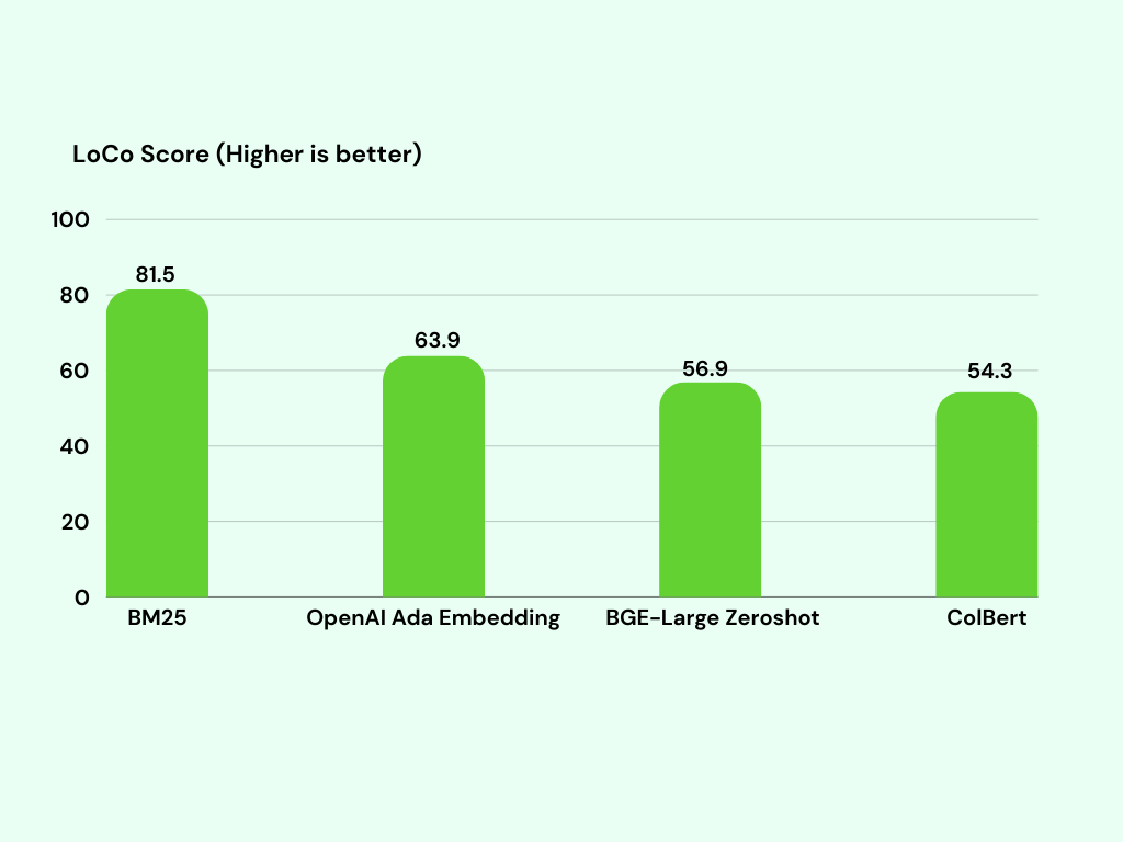
BM25 has been shown to outperform dense vector-based retrieval methods in numerous RAG benchmark tasks. By integrating BM25 into PostgreSQL, you can achieve superior search performance and relevance, especially for applications requiring high-quality text retrieval. You can also combine it with vector search as the hybrid search integration.
Key Features
-
BM25 Statistic Sparse Vectors: Generate BM25 sparse vectors for text based on your own text data.
-
Integration with Vector Search Extensions: Compatible with
pgvecto.rsandpgvectorfor efficient vector searches in PostgreSQL. -
Seamless Tokenization: Utilizes Huggingface’s
bert-base-uncasedvocabulary with Byte-Pair Encoding (BPE) tokenizer, boosting performance with subword tokenization
How Does It Work?
The BM25 computation can be decomposed into separate components for the query and the documents. The final relevance score is calculated as the dot product between the query’s sparse vector and the document’s sparse vector. Therefore we transform BM25 into a sparse vector retrieval problems with dot product distance!
Usage
Here’s a step-by-step overview of how it works:
-
Create BM25 Statistics: Use the
bm25_createfunction to generate BM25 statistics for your document set. This function takes the table name, column name, and a statistic name as parameters and creates a materialized view to store the BM25 statistics. -
Generate Document Sparse Vectors: Convert your document text into sparse vector representations using the
bm25_document_to_svectorfunction. This function takes the BM25 statistic name and the document text as inputs. -
Generate Query Sparse Vectors: For each search query, generate a corresponding sparse vector using the
bm25_query_to_svectorfunction. This function also takes the BM25 statistic name and the query text as inputs. -
Calculate Relevance Scores: Compute the relevance score of documents for a given query by performing a dot product between the query sparse vector and the document sparse vectors. This score indicates how well a document matches the query.
Join the Community
We invite you to try pg_bestmatch.rs and share your feedback. Your contributions and suggestions are invaluable as we continue to enhance and refine this extension. Star our GitHub repository and join our Discord server to get started and become part of our growing community and share your feedback with us.
Experience the power of BM25 text queries in PostgreSQL with pg_bestmatch.rs —your new go-to tool for efficient and accurate text retrieval.
1.26 - My binary vector search is better than your FP32 vectors
Within the field of vector search, an intriguing development has arisen: binary vector search. This approach shows promise in tackling the long-standing issue of memory consumption by achieving a remarkable 30x reduction. However, a critical aspect that sparks debate is its effect on accuracy.
We believe that using binary vector search, along with specific optimization techniques, can maintain similar accuracy. To provide clarity on this subject, we showcase a series of experiments that will demonstrate the effects and implications of this approach.
What is a binary vector?
A binary vector is a representation of a vector where each element in the vector is encoded as a binary value, typically either 0 or 1. This encoding scheme transforms the original vector, which may contain real-valued or high-dimensional data, into a binary format.
Binary vectors require only one bit of memory to store each element, while the original float32 vectors need 4 bytes for each element. This means that using binary vectors can reduce memory usage by up to 32 times. Additionally, this reduction in memory requirements corresponds to a notable increase in Requests Per Second (RPS) for binary vector operations.
Let’s consider an example where we have 1 million vectors, and each vector is represented by float32 values in a 3072-dimensional space. In this scenario, the original float32 vector index would require around 20 gigabytes (GB) of memory to store all the vectors.
Now, if we were to use binary vectors instead, the memory usage would be significantly reduced. In this case, the binary vector index would take approximately 600 megabytes (MB) to store all 1 million vectors.
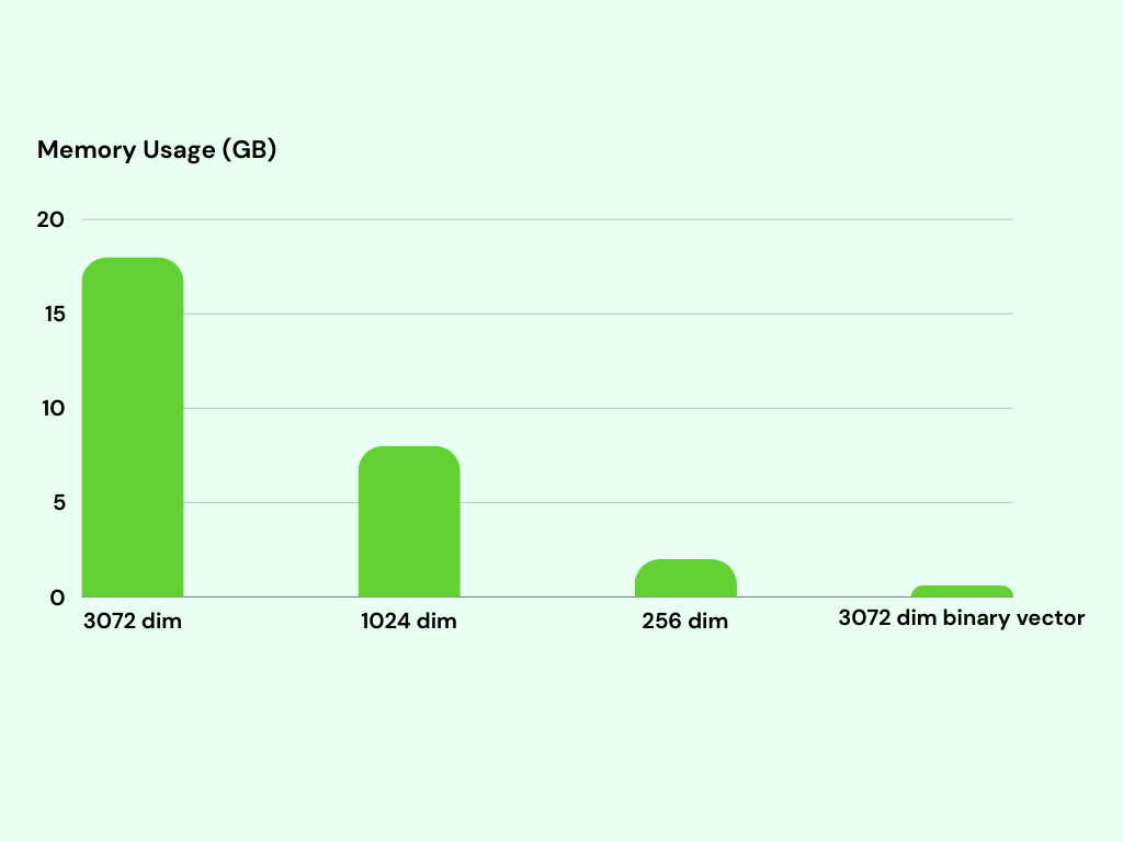
However, it was expected that this reduction in memory would lead to a significant decrease in accuracy because binary vectors lose a lot of the original information.
Surprisingly, our experiments showed that the decrease in accuracy was not as big as expected. Even though binary vectors lose some specific details, they can still capture important patterns and similarities that allow them to maintain a reasonable level of accuracy.
Experiment
To evaluate the performance metrics in comparison to the original vector approach, we conducted benchmarking using the dbpedia-entities-openai3-text-embedding-3-large-3072-1M dataset. The benchmark was performed on a Google Cloud virtual machine (VM) with specifications of n2-standard-8, which includes 8 virtual CPUs and 32GB of memory. We used pgvecto.rs v0.2.1 as the vector database.
After inserting 1 million vectors into the database table, we built indexes for both the original float32 vectors and the binary vectors.
After building the indexes, we conducted vector search queries to assess the performance. These queries were executed with varying limits, indicating the number of search results to be retrieved (limit 5, 10, 50, 100).
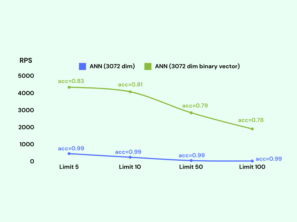
We observed that the Requests Per Second (RPS) for binary vector search was approximately 3000, whereas the RPS for the original vector search was only around 300.
The RPS metric indicates the number of requests or queries that can be processed by the system per second. A higher RPS value signifies a higher throughput and faster response time.
However, the accuracy of the binary vector search was reduced to about 80% compared to the original vector search. While this decrease may not be seen as significant in some cases, it can be considered unacceptable in certain situations where achieving high accuracy is crucial.
Optimization: adaptive retrieval
Luckily, we have a simple and effective method called adaptive retrieval, which we learned from the Matryoshka Representation Learning, to improve the accuracy.
The name is complex but the idea behind adaptive retrieval is straightforward. Let’s say we want to find the best 100 candidates. We can follow these steps:
-
Query the binary vector index to retrieve a larger set (e.g. 200 candidates) from the 1 million embeddings. This is a fast operation.
-
Rerank the candidates using a KNN query to retrieve the top 100 candidates. Please notice that we are running KNN instead of ANN. KNN is well-suited for scenarios where we need to work with smaller sets and perform accurate similarity search, making it an excellent choice for reranking in this case.
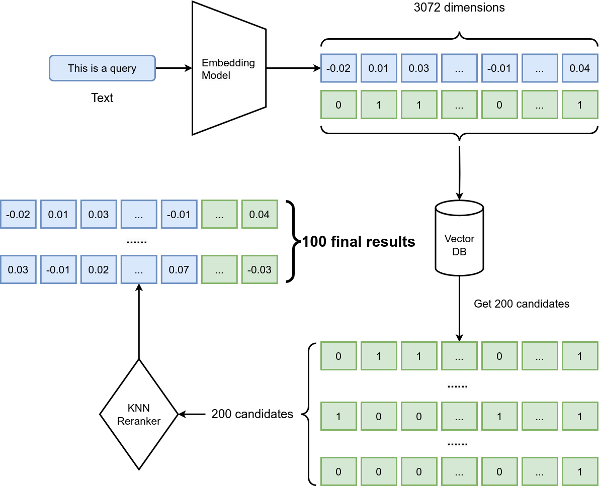
By incorporating this reranking step, we can achieve a notable increase in accuracy, potentially reaching up to 95%. Additionally, the system maintains a high Requests Per Second (RPS), approximately 1700. Furthermore, despite these improvements, the memory usage of the index remains significantly smaller, around 30 times less, compared to the original vector representation.
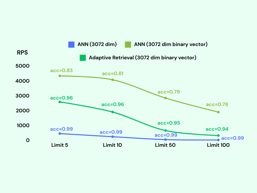
Below is the SQL code that can be used to execute the adaptive retrieval:
Comparison with shortening vectors
OpenAI latest embedding model text-embedding-3-large has a feature that allows you to shorten vectors.

It produces embeddings with 3072 dimensions by default. But you could safely remove some numbers from the end of the sequence and still maintain a valid representation for the text. For example, you could shorten the embeddings to 1024 dimensions.
This feature can help you save memory and make your requests faster, just like binary vectors. It would be a good idea to compare the performance and see which one works better for your needs.
Based on what we discovered, the conclusion is clear: Binary vectors significantly outperform shortened vectors.
We performed similar benchmarks to compare with binary vectors. We created indexes using the same dataset and machine type, but with varying dimensionalities. One index had 256 dimensions, while the other had 1024 dimensions.
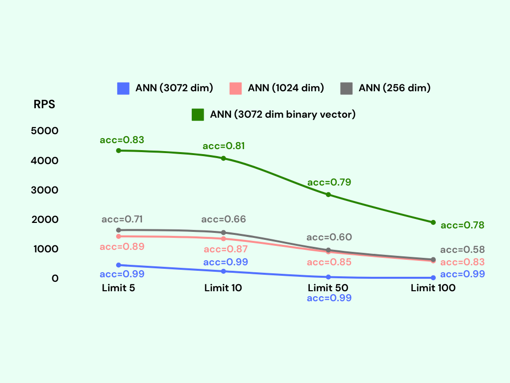
The 1024-dimensional index achieved an accuracy of approximately 85% with a request rate of 1000 requests per second (RPS). On the other hand, the 256-dimensional index had around 60% accuracy with a higher request rate of 1200 RPS.
The 1024-dimensional index required approximately 8GB of memory, while the 256-dimensional index used around 2GB. In comparison, the binary vector approach achieved an accuracy of around 80% with a request rate of 3000 RPS, and its memory usage was approximately 600MB.
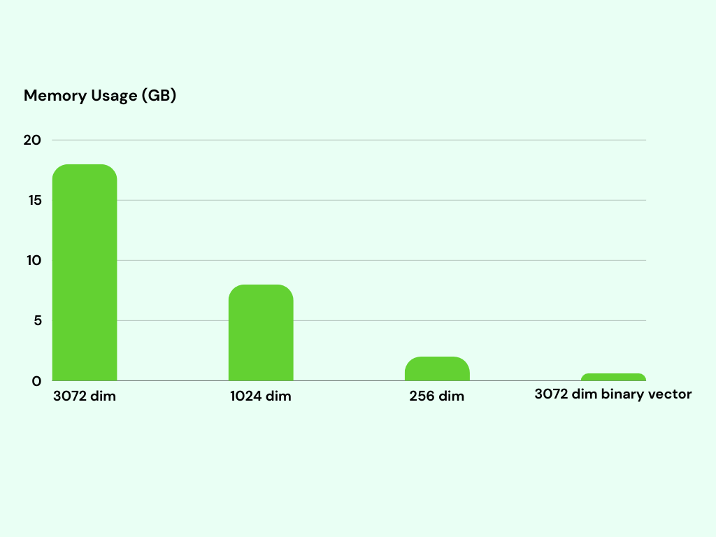
We implemented adaptive retrieval with lower-dimensional indexes. The binary vector index still outperformed the 256-dimensional index in terms of both request rate (RPS) and accuracy, while also exhibiting lower memory usage. On the other hand, the adaptive retrieval with the 1024-dimensional index achieved a higher accuracy of 99%; however, it had a relatively lower request rate and consumed 12 times more memory compared to the other indexes.
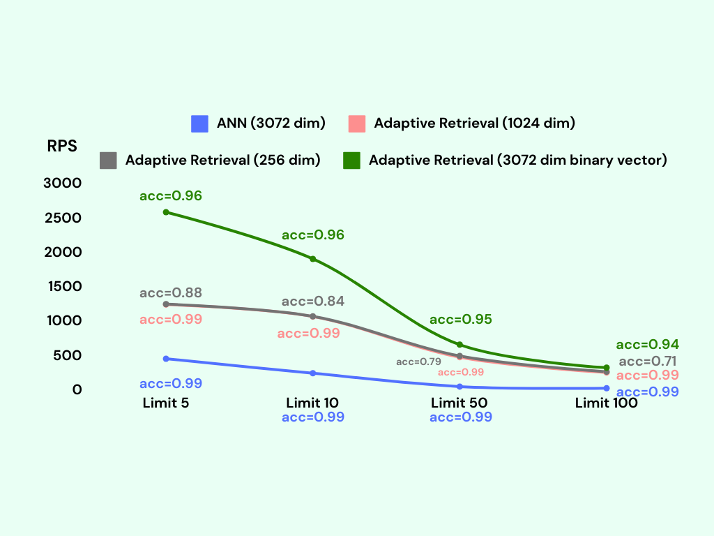
Summary
By utilizing adaptive retrieval techniques, binary vectors can maintain a high level of accuracy while significantly reducing memory usage by 30 times. We have presented benchmark metrics in a table to showcase the results. It is important to note that these outcomes are specific to the openai text-embedding-3-large model, which possesses this particular property.
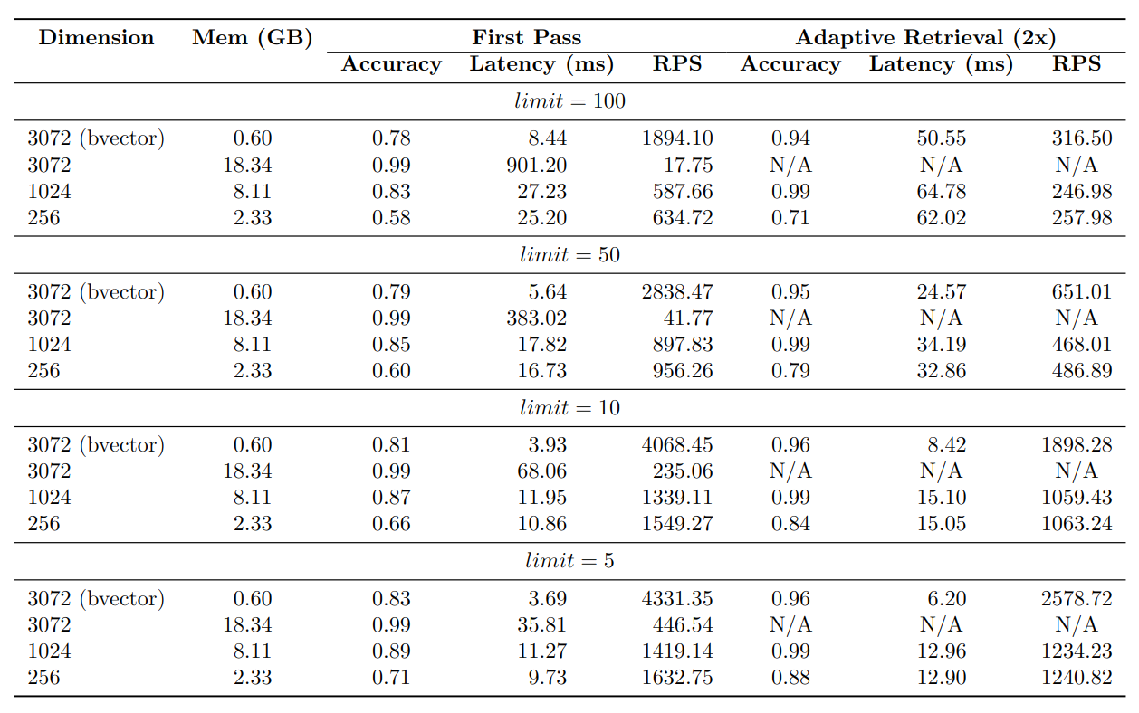
1.27 - pgvector vs. pgvecto.rs in 2024: A Comprehensive Comparison for Vector Search in PostgreSQL
pgvector and pgvecto.rs are both vector search extensions designed to enhance the capabilities of PostgreSQL. These extensions revolutionize the way vector search is performed within the database, providing scalable, low-latency, and hybrid-enabled solutions. In this blog post, we will illustrate the differences between pgvector and pgvecto.rs.
TL; DR: Please navigate directly to the final section that contains a table showcasing the main distinctions between the two.
Search
Search is essential for a database. It plays a pivotal role in facilitating efficient data retrieval, enabling users to quickly find and access the information they need. We will demonstrate their performance and highlight the various features pgvecto.rs and pgvector offer.
Filtering
While both pgvector and pgvecto.rs provide support for vector similarity search in PostgreSQL, pgvecto.rs goes a step further by introducing VBASE method from OSDI 2023.
Real-world workloads often involve a combination of vector search and relational queries. While vector search is powerful for similarity matching and retrieval of similar vectors, relational queries allow you to perform complex joins, filters, and aggregations on structured data.
pgvecto.rs is designed to perform efficiently in scenarios that involve Single-Vector TopK + Filter + Join.
We utilize the laion-768-5m-ip-probability dataset for benchmarking purposes due to the absence of a comprehensive relational benchmark. The dataset is derived from LAION 2B images. It contains 5,000,000 vectors, 10,000 queries.
The dataset includes a probability column that stores random floating-point values generated from a uniform distribution between 0 and 1. The ratio of 0.01 means that each query covers 1% (or 0.01 times) of the dataset, allowing for focused analysis.
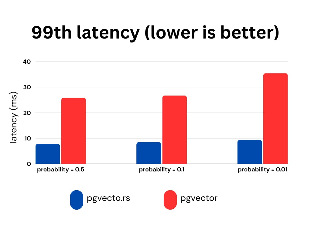
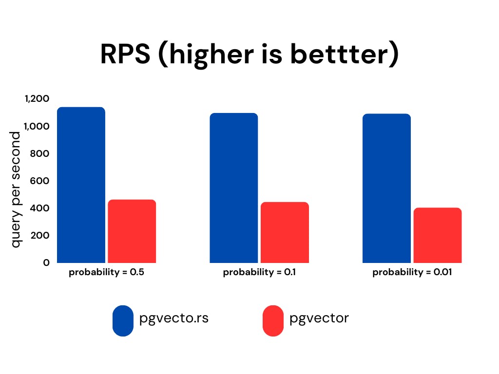
We present the recall, latency (in milliseconds), and RPS (requests per second) for various probability ranges while keeping the ef_search constant. The ef_search parameter represents the size of the list utilized during k-NN (k-Nearest Neighbors) searches, determining the trade-off between search accuracy and query processing time.
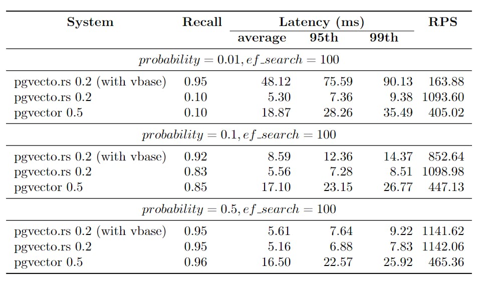
pgvecto.rs, when used with VBASE, consistently yields improved recall, particularly when working with low probability values.
Sparse Vector Search
Sparse vectors are high-dimensional vectors that contain few non-zero values. They are suitable for traditional information retrieval use cases. For example, a vector with 32,000 dimensions but only 2 non-zero elements is a typical sparse vector.
Dense vectors are embeddings from neural networks. They are generated by text embedding models and have most or all elements non-zero. They have fewer dimensions, such as 256 or 1536, much less than sparse vectors.
pgvector supports dense vector search well, but it does not have plan to support sparse vector.
pgvecto.rs, on the other hand, supports both dense vector search and sparse vector search. It provides the ability to use the svector data type to build sparse vector indexes and perform searches on them.
Vector dimensions
The pgvecto.rs extension provides support for up to 65535 dimensions, whereas the pgvector extension supports a maximum of 2000 dimensions. This difference in dimensionality support allows pgvecto.rs to handle vectors from OpenAI’s latest embedding model directly.
Single Instruction/Multiple Data (SIMD)
pgvecto.rs utilizes the SIMD (Single Instruction, Multiple Data) instructions available on the user’s machine, pgvector relies on the compiler to generate SIMD code at compile time and cannot choose a faster instruction set at runtime. It makes search in pgvecto.rs faster due to the faster calculation of vector distances.
Data Types
Binary Vector
The bvector type is a binary vector type in pgvecto.rs. It represents a binary vector, which is a vector where each component can take on two possible values, typically 0 and 1.
Binary vectors offer significant advantages in specific embedding models like the OpenAI embedding model by effectively reducing memory usage while preserving a satisfactory level of accuracy.
Here are some performance benchmarks for the bvector type. We use the dbpedia-entities-openai3-text-embedding-3-large-3072-1M dataset for the benchmark. The VM is n2-standard-8 (8 vCPUs, 32 GB memory) on Google Cloud.
We upsert 1M binary vectors into the table and then run a KNN query for each embedding. It only takes about 600MB memory to index 1M binary vectors, while the vector type takes about 18GB memory to index the same number of vectors. The bvector’s accuracy exceeds 95% if we adopt adaptive retrieval.

FP16/INT8
Besides binary vectors, pgvecto.rs also provides support for FP16 (16-bit floating point) and INT8 (8-bit integer) data types.
Indexing
pgvecto.rs takes a different approach compared to pgvector. It handles the storage and memory of indexes separately from PostgreSQL, instead of relying on the native storage engine of PostgreSQL like pgvector does.
It’s a design tradeoff. During the initial stages of our development, we conducted experiments with PostgreSQL’s page storage for the Hierarchical Navigable Small World (HNSW) index. similar to pgvector. However, we encountered various limitations that hindered its effectiveness and functionality:
-
Parallelization Challenges: The process model of PostgreSQL, where each statement corresponds to a single process and the lack of thread-safe APIs, presents challenges for parallelization. In the case of building vector indexes, which involve computationally intensive tasks, parallelization can significantly enhance performance. However, our efforts to parallelize this process were impeded by frequent occurrences of ‘Too many shared buffer locked’ errors.
-
Write-Ahead Logging (WAL) Amplification: The issue of Write-Ahead Logging (WAL) amplification arises when inserting a 2KB vector results in generating over 20KB of WAL. This problem is inherent in the HNSW algorithm used, as it involves modifying multiple edges for a single point insertion. PostgreSQL records each change individually in the WAL, leading to substantial amplification of the WAL size.
-
Lock Contention: Lock contention arises due to the need to lock every edge list during reads and writes when traversing the HNSW graph. The hierarchical structure of HNSW, where higher levels contain fewer points, often results in lock contention becoming a common bottleneck during index usage. This contention occurs when multiple operations attempt to access or modify the same edge list simultaneously, leading to delays and reduced concurrency.
pgvecto.rs adopted a design akin to FreshDiskANN, resembling the Log-Structured Merge (LSM) tree concept. This architecture comprises three components: the writing segment, the growing segment, and the sealed segment. New vectors are initially written to the writing segment. A background process then asynchronously transforms them into the immutable growing segment. Subsequently, the growing segment undergoes a merge with the sealed segment, akin to the compaction process in an LSM tree. This design offers several benefits:
-
Non-blocking Insertions: Index modification operations do not impede insertion processes.
-
Batched Modifications: Grouping modifications to the HNSW graph improves throughput.
-
Elimination of Read-Write Lock Contention: Since sealed segments are immutable, issues related to read-write lock contention are mitigated.
However, there are drawbacks to this approach. One notable limitation is the absence of out-of-the-box Write-Ahead Logging (WAL) support for the index. This means that features like Point-in-Time Recovery and Physical Replication, which rely on WAL, are not readily available for the index. Nevertheless, the PostgreSQL ecosystem is robust and allows for extensions to define their own custom WAL through a resource manager. While implementing this solution requires additional effort, it is feasible to overcome the limitation and enable WAL support for the index.
Summary
Here we will show the main distinctions between pgvecto.rs and pgvector.
| Feature | pgvecto.rs | pgvector |
|---|---|---|
| Filtering | Introduces VBASE method for vector search and relational query (e.g. Single-Vector TopK + Filter + Join). | When filters are applied, the results may be incomplete. For example, if you originally intended to limit the results to 10, you might end up with only 5 results with filters. |
| Sparse Vector Search | Supports both dense and sparse vector search. | Supports dense vector search. |
| Vector Dimensions | Supports up to 65535 dimensions. | Supports up to 2000 dimensions. |
| SIMD | SIMD instructions are dynamically dispatched at runtime to maximize performance based on the capabilities of the specific machine. | Relies on compiler-generated SIMD code at compile time. |
| Data Types | Introduces additional data types: binary vectors, FP16 (16-bit floating point), and INT8 (8-bit integer). | - |
| Indexing | Handles the storage and memory of indexes separately from PostgreSQL | Relies on the native storage engine of PostgreSQL |
| WAL Support | Provides Write-Ahead Logging (WAL) support for data, index support is working in progress. | Provides Write-Ahead Logging (WAL) support for index and data. |
1.28 - Building LLM Applications in LangChain using pgvecto.rs
LangChain is a framework for developing applications powered by language models. It enables applications that:
-
Are context-aware: connect a language model to sources of context (prompt instructions, few shot examples, content to ground its response in, etc.)
-
Reason: rely on a language model to reason (about how to answer based on provided context, what actions to take, etc.)
pgvecto.rs is a vector search extension in Postgres. In this blog post, we’ll show you how to build LLM applications with LangChain and pgvecto.rs.
Install dependencies
Some dependencies are required to use the LangChain integration:
You could start the postgres instance with pgvecto.rs extension in a docker container:
Then you can connect to the database using the psql command line tool. The default username is postgres, and the default password is mysecretpassword.
Run the following SQL to ensure the extension is enabled.
Create the database and load documents
We will show how to use pgvecto.rs in LangChain to retrieve the most similar vectors.
First, you need to create the text loader and the text splitter to split the text into chunks. We use the markdown file pgvecto-rs/getting-started/overview.md as an example.
Then, we will create the PGVecto_rs instance and load the documents into the database.
Query index
Finally, we can retrieve the most similar chunks in LangChain.
The output is:
Initialize from an existing database
Above, we created a vector store from scratch. However, often times we want to work with an existing vector store. In order to do that, we can initialize it directly.
Then, we can add vectors to the store and query:
The output is:
1.29 - Building the RAG pipeline with LlamaIndex and pgvecto.rs
LlamaIndex is a simple, flexible data framework for connecting custom data sources to large language models (LLMs).
pgvecto.rs provides a LlamaIndex integration that allows you to retrieve the most similar vectors. In this blog post, we will show you how to build a RAG pipeline with pgvecto.rs and LlamaIndex.
Install dependencies
Some dependencies are required to use the LlamaIndex integration:
You could start the Postgres instance with pgvecto.rs extension in a docker container:
Then you can connect to the database using the psql command line tool. The default username is postgres, and the default password is mysecretpassword.
Run the following SQL to ensure the extension is enabled.
Create the database and load documents
First, create the text loader and the text splitter to split the text into chunks. We use the markdown file pgvecto-rs/getting-started/overview.md as an example.
Then set up the OpenAI API key and load the documents into the database.
Query index
Finally, we can retrieve the most similar chunks.
1.30 - Do we really need a specialized vector database?
With the popularity of LLM (Large Language Model), vector databases have also become a hot topic. With just a few lines of simple Python code, a vector database can act as a cheap but highly effective “external brain” for your LLM. But do we really need a specialized vector database?
Why does LLM need vector search?
First, let me briefly introduce why LLM needs to use vector search technology. Vector search is a problem that has been around for a long time. The process of finding the most similar object in a collection given an object is vector search. Text/images, etc. can be converted into a vector representation, and the similarity problem of text/images can be transformed into a vector similarity problem.
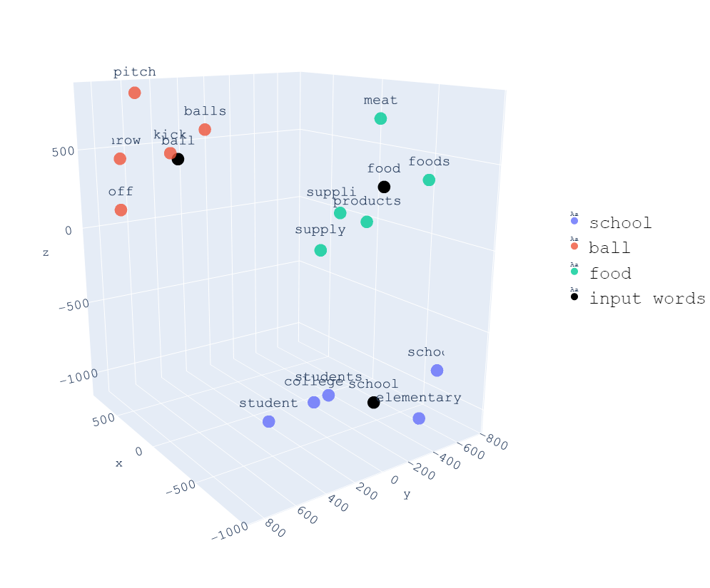
Text search (credit)
In the example above, we convert different words into a three-dimensional vector. Therefore, we can intuitively display the similarity between different words in a 3D space. For example, the similarity between “student” and “school” is higher than the similarity between “student” and “food”.
Returning to LLM, the limitation of the context window length is a major challenge. For instance, ChatGPT 3.5 has a context length limit of 4k tokens. This poses a significant problem for LLM’s context-learning ability and negatively impacts the model’s user experience. However, vector search provides an elegant solution to this problem:
-
Divide the text that exceeds the context length limit into shorter chunks and convert different chunks into vectors (embeddings).
-
Before inputting the prompt to LLM, convert the prompt into a vector (embedding).
-
Search the prompt vector to find the most similar chunk vector.
-
Concatenate the most similar chunk vector with the prompt vector as the input to LLM.
This is like giving LLM an external memory, which allows it to search for the most relevant information from this memory. This memory is the ability brought by vector search. If you want to learn more details, you can read these articles (Article 1 and Article 2), which explain it more clearly.
Why is vector database so popular?
In LLM, the vector database has become an indispensable part, and one of the most important reasons is its ease of use. After being used in conjunction with OpenAI Embedding models (such as text-embedding-ada-002), it only takes about ten lines of code to convert a prompt query into a vector and perform the entire process of vector search.
In LLM, vector search mainly plays a role in recall. Simply put, recall is finding the most similar objects in a candidate set. In LLM, the candidate set is all chunks, and the most similar object is the chunk that is most similar to the prompt. In the reasoning process of LLM, vector search is regarded as the main implementation of recall. It is easy to implement and can use OpenAI Embedding models to solve the most troublesome problem of converting text into vectors. The remaining part is an independent and clean vector search problem, which can be well completed by current vector databases. Therefore, the entire process is particularly smooth.
As the name suggests, vector database is a database specifically designed for the special data type of vectors. The similarity calculation of vectors was originally an O(n^2) complexity problem because it required comparing all vectors in the set pairwise. Therefore, the industry proposed the Approximate Nearest Neighbor (ANN) algorithm. By using the ANN algorithm, the vector index is constructed by pre-calculating in the vector database, using the idea of trading space for time, which greatly speeds up the process of similarity calculation. This is similar to the index in traditional databases.
Therefore, vector databases not only have strong performance but also excellent ease of use, making them a perfect match for LLM! (Really?)
Perhaps a general-purpose database would be better?
We’ve talked about the advantages and benefits of vector databases, but what are their limitations? A blog post by SingleStore provides a good answer to this question:
Vectors and vector search are a data type and query processing approach, not a foundation for a new way of processing data. Using a specialty vector database (SVDB) will lead to the usual problems we see (and solve) again and again with our customers who use multiple specialty systems: redundant data, excessive data movement, lack of agreement on data values among distributed components, extra labor expense for specialized skills, extra licensing costs, limited query language power, programmability and extensibility, limited tool integration, and poor data integrity and availability compared with a true DBMS.
There are two issues that I think are important. The first is the issue of data consistency. During the prototyping phase, vector databases are very suitable, and ease of use is more important than anything else. However, a vector database is an independent system that is completely decoupled from other data storage systems such as TP databases and AP data lakes. Therefore, data needs to be synchronized, streamed, and processed between multiple systems.
Imagine if your data is already stored in an OLTP database such as PostgreSQL. To perform vector search using an independent vector database, you need to first extract the data from the database, then convert each data point into a vector using services such as OpenAI Embedding, and then synchronize it to a dedicated vector database. This adds a lot of complexity. Furthermore, if a user deletes a data point in PostgreSQL but it is not deleted in the vector database, then there will be data inconsistency issues. This issue can be very serious in actual production environments.
On the other hand, if everything is done in a general-purpose database, the user experience may be simpler than with an independent vector database. Vectors are just one data type in a general-purpose database, not an independent system. This way, data consistency is no longer an issue.
The second issue is with query language. The query language of vector databases is typically designed specifically for vector search, so there may be many limitations in other types of queries. For example, in metadata filtering scenarios, users need to filter based on certain metadata fields. The filtering operators supported by some vector databases are limited.
In addition, the supported data types for metadata are also very limited, usually only including String, Number, List of Strings, and Booleans. This is not friendly for complex metadata queries.
If traditional databases can support the vector data type, then the aforementioned issues do not exist. Firstly, data consistency is already taken care of as TP or AP databases are existing infrastructure in production environments. Secondly, the issue of query language no longer exists because vector data type is just one data type in the database, so queries for vector data type can use the native query language of the database, such as SQL.
Detailed explanation
However, it is unfair to only compare the disadvantages of vector databases. There are several counterpoints to consider:
-
Ease of Use: Vector databases are designed with ease of use in mind, and users can easily work with them without worrying about the underlying implementation details. However, integrating them with other data storage systems can be a challenge, as mentioned earlier.
-
Performance: Vector databases have a significant advantage over traditional databases in terms of performance for certain use cases. Their design for vector search allows for fast and efficient similarity searches on large-scale datasets with high-dimensional vectors.
-
Metadata Filtering: While metadata filtering capabilities in vector databases may be limited, they can still meet the needs of most business scenarios. However, for more complex metadata queries, a hybrid approach may be needed, where metadata is stored in a separate database or data lake and linked to the vector data in the vector database.
How can you address these issues? In the following section, I will provide my perspective by answering these questions.
Vector databases are easy to use
While it is true that vector databases are easy to use, this is not unique to them. The ease of use of vector databases is mainly due to their abstraction of a specific domain, which allows them to be specifically designed for the most commonly used machine learning programming language, Python, and optimized for vector search scenarios. However, if traditional databases could also support the vector data type, they could offer similar ease of use.
In addition, traditional databases can provide Python SDKs and other integrated tools to meet the needs of most scenarios, as well as standard SQL interfaces to handle more complex query scenarios. Therefore, it is not necessary to use a vector database solely for its ease of use.
Another advantage of vector databases is their distributed design, which allows them to scale horizontally to meet the data volume and QPS requirements of users. However, traditional databases can also meet these requirements through distributed systems. Nevertheless, the decision to use a distributed system should be based on the actual needs of the data volume and QPS requirements, as well as the associated costs.
In summary, while vector databases have their advantages, traditional databases can also provide similar ease of use and distributed capabilities if they support the vector data type. Therefore, the choice between a vector database and a traditional database should be based on the specific needs of the application and the available resources.
Vector databases have better performance
To investigate the performance of vector databases in LLM scenarios, a naive benchmark of vector retrieval was conducted. The benchmark involved N randomly initialized 256-dimensional vectors, and the query time for the top-5 nearest neighbors was measured for different scales of N. Two different methods were used for the test:
-
Numpy was used to perform real-time calculations, which executed completely accurate, non-precomputed nearest neighbor calculations.
-
Hnswlib was used to precompute approximate nearest neighbors.
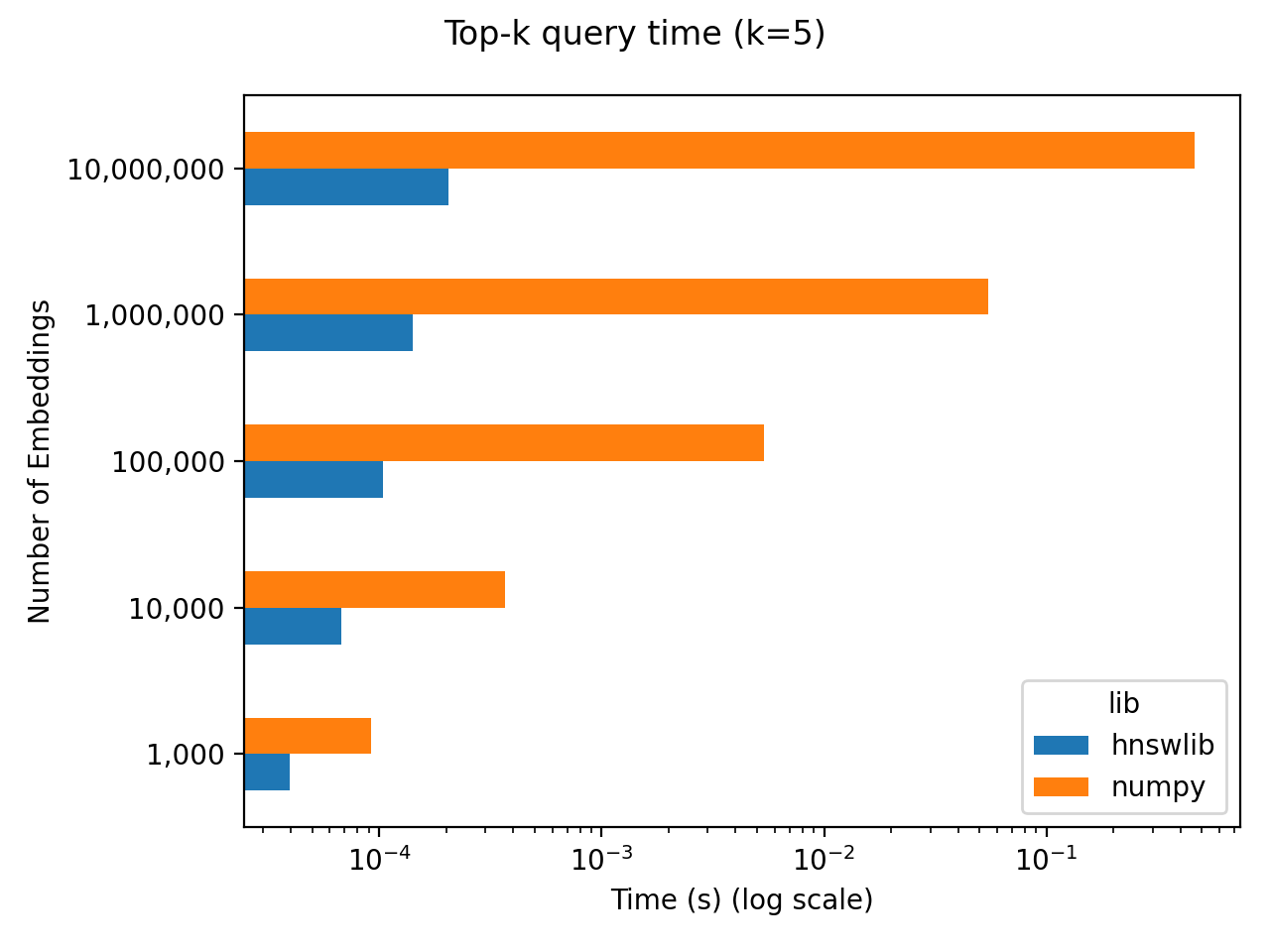
Benchmark (credit)
The benchmark results show that, at the scale of 1 million vectors, the delay of real-time calculation using Numpy is approximately 50ms. Using this as a benchmark, we can compare the time spent on LLM inference after completing vector search. For instance, the 7B model requires approximately 10 seconds for inference on 300 Chinese characters on an Nvidia A100 (40GB). Therefore, even if the query time for real-time accurate calculation of the similarity of 1 million vectors using Numpy is considered, it only accounts for 0.5% of the total delay in the end-to-end LLM inference. Thus, in terms of delay, the benefits brought by vector databases may be overshadowed by the delay of LLM itself in the current LLM scenario. Therefore, we need to also consider throughput. The throughput of LLM is much lower than that of vector databases. Thus, I do not believe that throughput is the core issue in this scenario.
If performance is not the primary concern, what factors will determine the user’s choice? I think it is the overall ease of use, including ease of use for both usage and operation, consistency, and other solutions to database-related issues. Traditional databases have mature solutions for these problems, while vector databases are still in the early stages of development.
Metadata filtering can still meet the needs of most business scenarios
When considering metadata filtering, it’s important to note that it’s not just a matter of the number of supported operators. Consistency of data is also a crucial factor. Metadata in vectors is essentially data in traditional databases, while vectors themselves are indexes of the data. Therefore, it’s reasonable to consider storing both vectors and metadata in traditional databases.
Traditional databases do have the capability to support vector data types and provide similar ease of use and distributed capabilities as vector databases. Furthermore, traditional databases have mature solutions to ensure data consistency and integrity, such as transaction management and data backup and recovery.
Vectors in traditional databases
Since we see vectors as a new data type in traditional databases, let’s take a look at how to support vector data types in traditional databases, using PostgreSQL as an example. pgvector is an open-source PostgreSQL plugin that supports vector data types. pgvector uses exact calculation by default, but it also supports building an IVFFlat index and precomputing ANN results using the IVFFlat algorithm, sacrificing calculation accuracy for performance.
pgvector has done an excellent job of supporting vectors and is used by products such as supabase. However, the supported index algorithm is limited, with only the simplest IVFFlat algorithm supported, and no quantization or storage optimization is implemented. Moreover, the index algorithm of pgvector is not disk-friendly and is designed for use in memory. Therefore, vector index algorithms designed for disk, such as DiskANN, are also valuable in the traditional database ecosystem.

Extending pgvector can be challenging due to its implementation in the C programming language. Despite being open-source for two years, pgvector currently has only three contributors. While the implementation of pgvector is not particularly complex, it may be worth considering rewriting it in Rust.
Rewriting pgvector in Rust can enable the code to be organized in a more modern and extensible way. Rust’s ecosystem is also very rich, with existing Rust bindings such as faiss-rs.
pgvecto.rs
As a result, pgvecto.rs was created. pgvecto.rs currently supports exact vector query operations and three distance calculation operators. Work is underway to design and implement index support. In addition to IVFFlat, we also hope to support more indexing algorithms such as DiskANN, SPTAG, and ScaNN. We welcome contributions and feedback from the community!
pgvecto.rs offers a modern and extensible codebase with improved performance and concurrency. Its design and implementation allow seamless integration with other machine learning libraries and tools, making it an ideal choice for similarity search scenarios.
With ongoing development, pgvecto.rs aims to be a valuable tool for data scientists and machine learning practitioners. Its support for various indexing algorithms and its ease of use make it a promising candidate for large-scale similarity search applications. We look forward to continuing development and contributions from the community.
Future
As LLMs gradually move into production environments, infrastructure requirements are becoming increasingly demanding. The emergence of vector databases is an important addition to the infrastructure. We do not believe that vector databases will replace traditional databases, but rather that they will each play to their strengths in different scenarios. The emergence of vector databases will also promote traditional databases to support vector data types.
We hope that pgvecto.rs can become an important component of the Postgres ecosystem, providing better vector support for Postgres. Its implementation in Rust and support for various indexing algorithms make it a promising candidate for large-scale similarity search applications. We believe that its development and contributions from the community will help it become a valuable tool for data scientists and machine learning practitioners.
2 - Release Notes
2.1 - VectorChord 1.1: Native 4/8 Bit Vector Types and Per-Index Query Defaults
We’re excited to announce the release of VectorChord 1.1 as we kick off the new year of horse.
VectorChord 1.0 was a milestone for Postgres-native vector search: it made large-scale indexing fast enough to feel like iteration, not an outage. In 1.1, we’re building on that foundation with RaBitQ8: A new vector type that delivers 4x storage savings and faster search speeds compared to float32, all with less than 1% recall loss. Paired with RaBitQ4 and more composable query control, VectorChord 1.1 is ready for your most demanding production workloads.
This release focuses on two pain points we’ve observed through community feedback:
-
Capacity constraints. When vector indexes grow massive, scaling isn’t just about throughput. It is also about SSD footprint and buffer cache pressure.
-
Operational Overhead. As the number of indexes grows, manually setting search parameters (like nprobe) for every query clutters your application logic. This becomes a major headache in scenarios like partitioned tables, where individual indexes need distinct configurations. Relying on a global session variable (GUC) makes it impossible to tune these indexes independently.
VectorChord 1.1 addresses both. We’re introducing rabitq8 and rabitq4, native quantized vector types that are 4x and 8x smaller than standard float32. These types shrink total index size by 4x–7x, drastically reducing storage overhead. We’ve also added per-index query defaults, allowing multi-index queries to rely on specific configurations rather than a brittle global PostgreSQL GUC.
RaBitQ8 & RaBitQ4: Low bit vector type for storage efficiency
Vector data footprint is the hidden limiter of large-scale search on Postgres. Storing high-dimensional vectors as standard float32 (4 bytes per dimension) consumes massive amounts of SSD space and memory. As this footprint grows, it increases buffer cache pressure and forces queries to read from disk, causing P99 latency to spike.
VectorChord 1.1 solves this with two new quantized data types: rabitq8 and rabitq4, built on extended RaBitQ (paper). By using 8-bit and 4-bit representations instead of 32-bit floats, these types reduce per-vector storage by 4x and 8x respectively, while keeping accuracy loss minimal.
Using these types is almost identical to using vector. The only difference is that you quantize values with quantize_to_rabitq8 or quantize_to_rabitq4 during INSERT and SELECT.
On LAION with 100M 768-dimensional vectors, a typical vector (float32) index occupies about 400GB. Using the halfvec (float16) type reduces that to roughly 171GB. Under the same index options, switching to rabitq8 further reduces it to about 95GB, and rabitq4 to around 58GB, delivering a 4x to 7x footprint reduction compared with the baseline.

The next question is the recall and throughput trade-off. rabitq8 delivers the index size reduction while keeping recall and QPS essentially on par with the baseline (float32 vectors). rabitq4 is a more aggressive option. It trades a larger recall loss for the smallest possible index size, and is best suited for deployments where storage is the primary constraint.

Per-Index Query Defaults: Composable Multi-Index Queries
In VectorChord, the vchordrq.probes GUC controls how much of the vector space is searched at query time, directly trading off throughput against recall. For hierarchical vchordrq indexes, vchordrq.probes must have the same length as the build.internal.lists configuration used at build time. Typical configurations look like:
build.internal.lists |
vchordrq.probes |
|
|---|---|---|
| No partition | [] |
'' |
| 1-layer partition | [2000] |
'40' |
| 2-layer partition | [800, 640000] |
'40,200' |
For simple vector search on a single table with a single index, setting the GUC once before running a query is a natural choice.
However, the situation changes when a single query touches more than one vector index. Indexes built with different build.internal.lists configurations should logically use different probes settings. Worse, when the number of list levels differs, no single global probes value can simultaneously match both indexes, making the global setting inherently unsuitable for such queries.
To solve this, VectorChord 1.1 introduces per-index query defaults as index options, following PostgreSQL’s per-index configuration model. Instead of forcing every query to share a single global configuration, each index can now define its own defaults, which take effect when a global configuration is not explicitly set.
You can set per-index defaults at index creation time, and modify them at any time without rebuilding the index.
In addition to vchordrq.probes, other query-time parameters can also be given per-index defaults at index creation time, so multi-index queries can rely on independent, index-specific settings. For the full list of configurable parameters, see Fallback Parameters.
Summary
VectorChord 1.1 makes large-scale deployments easier to run. rabitq8 and rabitq4 significantly reduce storage size, lowering storage and memory pressure while preserving a familiar SQL usage pattern. Per-index fallback query defaults make multi-index vector queries possible within a single statement, especially when those indexes are built with different options.
Whether you are hitting storage and memory limits in real-world workloads or running complex queries with multiple vector indexes, we invite you to upgrade to VectorChord 1.1, try it on your own workloads, and share your feedback.
-
Download/Star on GitHub: https://github.com/tensorchord/VectorChord
-
Join the Community: https://discord.gg/KqswhpVgdU
2.2 - VectorChord 1.0: Developer-First Vector Search on Postgres, 100x Faster Indexing than pgvector
Two years ago, when we published the very first pgvecto.rs blog post, we made a bet: Postgres is the best place to do vector search. Since then we’ve been iterating on that bet — from VBASE with filtered vector search, to longer vector support, to the RaBitQ quantization scheme and disk‑friendly index layouts.
With VectorChord 1.0 we’re moving the needle again. On a 16 vCPU machine, we can now build an index over 100M vectors in under 20 minutes. On the same scale, pgvector needs more than 50 hours. That number sounds impressive, but the point of this release isn’t just to win a benchmark slide. It’s to make your actual development and iteration loop much faster.
This post is organized into three parts:
1. Simplicity over complexity: breaking the “HNSW is always better” myth
When people first talk to us about VectorChord, one of the most common questions is very direct:
“Are you using HNSW? I heard HNSW is always better than IVF.”
On paper, HNSW is a beautiful algorithm. In many isolated benchmarks it wins. But we don’t run vector search inside a vacuum — we run it inside Postgres, with its own storage model, vacuuming, MVCC, and operational habits.
If you look at it from that angle, the trade‑off changes a lot.
The Postgres reality of HNSW
HNSW uses a layered graph structure. Every new vector is a node that may connect to several other nodes across multiple layers. Every delete potentially removes a node that many other nodes depend on.
In a stand‑alone vector engine you can design the entire storage engine around this structure. Inside Postgres, you can’t. You have to live inside the existing table/index model, work with vacuum, and behave well under MVCC.
That’s where the pain starts:
-
Insertions are heavy. Inserting a single vector into an HNSW index can trigger cascades of changes across multiple nodes and layers. Under high write load this makes it harder to keep latency stable.
-
Deletions are subtle. In practice, a delete often just marks a node as dead but leaves it in the graph so connectivity isn’t broken immediately. As more nodes are marked this way, search still walks through them, which adds extra latency when a large fraction of the graph is “dead but still present.”
-
Vacuum pays the real price. You can’t simply drop those nodes, because removing them outright would break neighborhoods and disconnect parts of the graph. To fix that, pgvector has to reinsert all the neighbors of a dead node so the graph stays connected without it. That reinsertion work is what makes maintenance expensive; the core issue isn’t just reclaiming dead tuples, it’s re‑wiring the graph around every deleted node.
None of this is impossible, but it pushes you toward high cost whenever you have frequent updates.
Why we chose IVF + RaBitQ instead
VectorChord’s core index is IVF + RaBitQ with simple posting lists. Vectors are routed into coarse clusters, and inside each cluster we store a tiny quantized code instead of a 768‑dimensional float. At query time almost all the work happens on these bit‑packed codes, using table lookups and cheap integer math.
Because the index mostly scans compressed codes, a posting‑list scan stays fast even when it touches many entries. In our benchmarks this makes VectorChord clearly faster than a naïve IVF that compares full‑precision vectors, and still faster than pgvector’s HNSW index, which walks its graph and scores neighbors with full‑precision arithmetic.
People sometimes ask “what about HNSW + quantized vectors?” You can do that, and it can speed up the first phase of a search, where you traverse the quantized vectors and pick candidates. But you still need a second phase that fetches and scores full‑precision vectors based on those candidates, and that part doesn’t care which index you used. In typical workloads the first phase is only about 40% of total latency, so even a 2x faster scan would only cut end‑to‑end time by roughly 20% — and because HNSW can’t lay out data in the tight, batch‑friendly fast‑scan format, even that theoretical gain may be hard to realize in practice.
With IVF + RaBitQ the postings are just arrays of compressed entries. Inserts append a new code; deletes clear a code. There is no global graph to repair, so frequent updates don’t trigger cascades of work. Operationally it behaves like a normal index, and in our tests this design handles around 10x the update throughput of pgvector’s HNSW index while keeping latency stable. For additional performance numbers — especially around query performance — please see our earlier blogs Vector Search Over PostgreSQL: A Comparative Analysis of Memory and Disk Solutions.
Most importantly, this simplicity is what enables the improvements in the next sections. If your index structure is already incredibly intricate, every extra optimization adds more moving parts. By keeping the core design simpler, we gave ourselves room to make index builds and developer workflows dramatically better.
2. Making indexing feel like iteration, not an outage
Let’s talk about the number in the title: 100x faster indexing than pgvector.
On paper, the comparison looks like this on LAION 100M‑vector dataset:
-
pgvector: more than 50 hours of index build time on 16 vCPUs (and it may fail if memory is insufficient).
-
VectorChord 0.1: KMeans done externally in about 2 hours on a GPU; insertion in Postgres taking around 20 hours on 4 vCPUs.
-
VectorChord 1.0: KMeans and insertion both done inside Postgres, finishing in under 20 minutes on 16 vCPUs (about 8 minutes for KMeans + 12 minutes for insertion).
But what changes for you is much simpler:
-
In the pgvector world, indexing a large dataset is a multi‑day event. You plan around it, you babysit it, you worry about what happens if it fails.
-
In the VectorChord 1.0 world, a full rebuild is closer to “run it before lunch and check the results after coffee.”
We got there by attacking both phases of IVF building: the KMeans step that finds centroids, and the insertion step that assigns every vector to its nearest centroid.
To get there, we tackled the problem instead of just the code. First, instead of micro‑optimizing a naïve 768‑dimensional, 160,000‑centroid KMeans over 100M points, we project vectors down to a much smaller space with Johnson–Lindenstrauss Lemma, which cuts the KMeans compute and memory footprint by roughly 7x. Second, we run hierarchical KMeans in two stages so we only ever cluster smaller subsets of the data instead of 160,000 centroids at once, which accelerates 400x in theory. For insertion, we reuse the same idea one level up by building an IVF over the centroids themselves, so each data vector only compares against a small set of candidate centroid buckets using quantized codes. Together these changes move most of the work out of CPU‑bound distance math: for a 100M‑vector build the dominant cost becomes Postgres allocating and writing index pages at roughly the SSD limit. After tightening the allocation path and lock granularity so we can stream pages out in large chunks, the practical result is that a full rebuild fits comfortably into minutes instead of days. For more details, we’ve written a dedicated blog How We Made 100M Vector Indexing in 20 Minutes Possible on PostgreSQL to explain the technical detail.
These optimizations can be done easily with the following SQL:
3. Features built for developers, not just for a benchmark chart
VectorChord 1.0 also adds a set of features that barely show up in benchmarks, but matter a lot when you live with the system every day. They’re all about helping you understand how your index behaves, and about letting you use modern models and deployments without friction.
Built‑in monitoring of index quality
All approximate nearest‑neighbor indexes drift over time. Data distributions change, and what was a great index at build time might quietly degrade.
Instead of leaving you to guess, VectorChord can continuously measure recall for you. It automatically samples real query vectors, re‑evaluates their neighbors with a more exact method, and tracks how often the index returns the “right” answers.
This turns a vague feeling — “search seems a bit off lately” — into a graph you can look at. If recall is steady, you know you can postpone a rebuild. If it’s trending down, you can plan a rebuild before users notice. It also gives you something concrete to feed into your existing observability stack, or into Prometheus so you can keep an eye on recall on the same dashboards as your other SLOs.
In practice, you can evaluate recall for a real query pattern with a single SQL call, and then export that number as a metric. For example:
Long vector support so you don’t have to cripple your model
We support vectors up to 16,000 dimensions. That sounds like a dry specification, but it has a clear practical effect: you can plug in newer models, including long‑context or multimodal ones, without immediately needing to compress or truncate their outputs just to make the index happy.
You can start with the representation your model naturally produces, get a feel for performance and quality, and then decide whether you want to apply more aggressive quantization or dimensionality reduction. The index shouldn’t be the thing forcing you to compromise on model choice.
Multi‑vector retrieval for richer RAG
Not every document fits into a single vector. Modern retrieval‑augmented generation (RAG) systems often represent a passage as a set of vectors — for example, one per token or one per sentence — and then compare that set to a set of query vectors. This “late interaction” style is usually called multi‑vector retrieval.
VectorChord supports this pattern natively via a MaxSim‑style operator over arrays of vectors. Conceptually, for each query vector you look for the best‑matching document vector, take their dot product, and then sum those best scores. In VectorChord this is exposed as the distance‑based @# operator on vector[] columns: the left‑hand side is the document’s vector array, the right‑hand side is the query’s vector array.
Getting started looks very similar to single‑vector search. You store an array of vectors per row and build a dedicated index:
At query time you pass in an array of query vectors and order by the @# score:
Under the hood VectorChord applies its ANN machinery to these vector arrays, so you get the expressiveness of multi‑vector models with the same kind of performance you expect from single‑vector IVF indexes — all inside Postgres and plain SQL.
Multi‑platform SIMD
VectorChord ships with SIMD acceleration for x86_64, ARM and IBM architectures. At runtime we detect the best available instruction set — AVX512 and friends where available — and use it without you having to tune build flags or keep separate binaries.
Experimental DiskANN + RaBitQ
We also have an experimental index type combining DiskANN with 2‑bit RaBitQ. On some datasets and recall targets it can deliver higher QPS than IVF + RaBitQ. The trade‑off is that indexing and updates are noticeably slower and more complex.
We don’t recommend this as the default choice. It’s there for teams who have very specific workloads, know exactly what they are doing, and are willing to pay higher operational costs for more QPS in a narrow slice of the parameter space. For everyone else, IVF + RaBitQ remains the recommended workhorse.
Similarity filters that stop scanning early
Sometimes you don’t just want the nearest neighbors; you want “everything within this radius, up to N rows.” The most natural way to write that in SQL is with a distance in the WHERE clause, plus ORDER BY and LIMIT:
This returns the right answers, but it performs poorly when only a few points fall inside the radius. Postgres still has to keep scanning the index until it finds ten rows or exhausts the search space, because the distance check is just a filter applied after the ANN scan.
VectorChord adds a “similarity filter” syntax that lets the distance threshold be pushed down into the index itself. You wrap the query vector and radius in a sphere() value, and use the <<->> operator so the index knows it can stop as soon as the search region moves beyond that sphere:
Prefilter and postfilter so queries match your data model
In real applications, vector search almost never happens in isolation. You filter by tenant, permissions, time ranges, or content type, then rank by vector similarity, or sometimes the other way around.
VectorChord lets you choose between prefiltering and postfiltering at the index level. In low‑selectivity scenarios, prefiltering can reduce the candidate set enough to get up to roughly five‑fold QPS improvements. In other cases you might want to search first and filter only the top results for better recall. The important part is that you can express both patterns naturally in Postgres.
Enabling prefiltering for a session is a single SQL statement:
Text search with VectorChord‑BM25
Finally, we added a VectorChord‑BM25 extension that brings strong text search directly into your Postgres instance. It supports multiple languages and advanced tokenization, and aims to be competitive with ElasticSearch‑style relevance for many workloads.
The idea is not to replace every dedicated search engine, but to let you build systems where BM25 and vector search live side by side, inside the same database, using the same operational tools. For many teams that alone removes a lot of deployment and maintenance burden.
In practice you can call it from plain SQL, combine it with your embeddings, and order by a unified score. For example:
Closing thoughts
VectorChord 1.0 is easy to summarize as “100x faster indexing than pgvector on 100M vectors.” That headline is true, but it is not the main story.
Our goal is to make VectorChord one of the best ways to do retrieval on Postgres, from the first prototype to billion‑scale datasets. If you’re already using pgvector, we’d love you to try VectorChord 1.0 on your real workloads and tell us where it helps and where it can do better. We would also like to express our appreciation to the EnterpriseDB team for their valuable feedback throughout this work.
2.3 - VectorChord 0.5: New RaBitQ-empowered DiskANN Index and Continuous Recall Measurement
We’re thrilled to announce the release of VectorChord 0.5! This release marks a significant step forward in our mission to provide more flexible, powerful, and controllable vector search capabilities. In the 0.5 release, we’re introducing two major updates: experimental support for the DiskANN graph index and a new recall measurement tool to monitor the health of your IVF+RaBitQ indexes proactively.
New Index Preview: RaBitQ-empowered DiskANN Index
From day one, VectorChord’s core indexing solution has relied on a powerful combination: the cluster-based IVF algorithm and RaBitQ quantization—what we ship as vchordrq (IVF+RaBitQ). This approach consistently delivers excellent low-latency, high-recall performance across a wide range of use cases and remains our recommended default for most scenarios.
At the same time, we recognize that graph-based indexes can outperform IVF+RaBitQ on certain datasets and at specific (often higher) recall targets. To give you the best tool for every job—and because our goal is to be a one‑stop solution for vector search—VectorChord 0.5 introduces experimental support for the DiskANN algorithm as an additional option.
What is DiskANN and Why Does It Matter?
Traditional top-tier graph algorithms (like HNSW and NSG) achieve their speed by keeping the entire graph in memory, which drives up hardware costs and caps single-node scale. SSDs are cheaper, but historically their random I/O made on-disk graphs impractical without big latency penalties.
DiskANN’s mission is to break this memory barrier. It’s a graph ANN designed from the ground up to store and search billion-scale datasets on inexpensive SSDs while maintaining competitive recall and low latency.
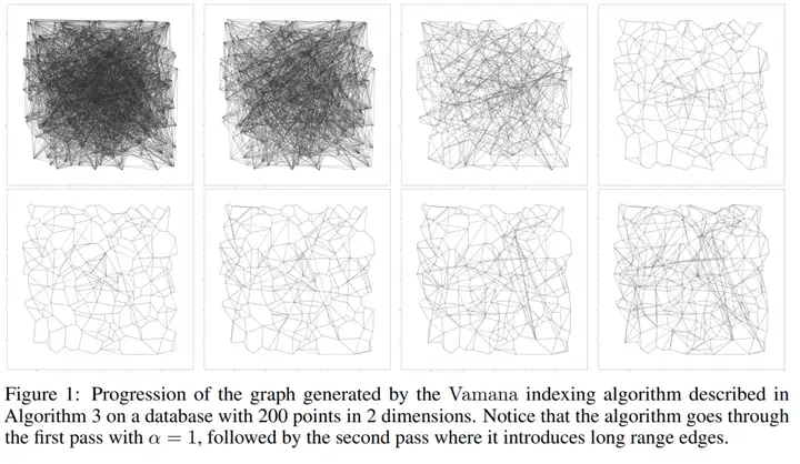
A visualization from the original DiskANN paper.
How our variant differs
We implement a variant of the original DiskANN design: instead of the paper’s default Product Quantization (PQ), our implementation uses RaBitQ as the quantization layer. RaBitQ is more accurate and comes with theoretical guarantees, which helps us deliver better recall–latency trade‑offs compared with vanilla PQ used in original implementations. In practice, this change enables stronger accuracy at the same footprint or faster queries at the same recall.
In VectorChord 0.5, we’ve integrated DiskANN into the existing ecosystem so you can evaluate it side-by-side with vchordrq.
When DiskANN Can Shine
-
Workload + target dependent gains. For some model families (e.g., OpenAI/Cohere‑style embeddings) and high-recall settings, DiskANN can deliver lower latency and/or higher recall than IVF+RaBitQ on the same hardware.
-
Stable and predictable build memory. It avoids the KMeans phase of IVF, reducing memory fluctuations during index build and simplifying capacity planning.
-
Ecosystem compatibility. Keep using VBase for metadata filtering and RaBitQ quantization for smaller footprint and faster re-ranking.
Important Considerations (Read This First)
DiskANN is still experimental in VectorChord, and—like all graph ANN methods—it entails trade‑offs:
-
Updates & build speed. Index builds and updates are much slower than with vchordrq (IVF+RaBitQ). If you have frequent inserts/deletes or need fast rebuilds, vchordrq is the better fit.
-
Dynamic data performance. Modifying graph connectivity is computationally heavier than updating IVF lists; expect better operational ergonomics with vchordrq for mutable datasets.
-
Operational simplicity. vchordrq tends to be simpler to tune and operate for most teams.
Our recommendation: Start with vchordrq (IVF+RaBitQ) for the majority of use cases. Consider DiskANN when you’re chasing top‑tier recall on relatively static corpora, want tighter tail latency at high recall, or when build‑time memory predictability is a hard requirement. Your feedback will help us harden this option for production.
How to Get Started
Check out our official documentation for detailed instructions on configuring and using the new graph index: Guide to Using Graph Index in VectorChord
Proactive Monitoring: Recall Measurement Tool for IVF+RaBitQ
A potential challenge with vector search index is “data distribution drift”. As you continuously add new data—especially when the new data’s vector distribution differs significantly from the initial dataset—the index’s recall can degrade over time, impacting query quality.
Previously, quantifying this degradation was difficult, often relying on intuition or complex offline evaluations to decide when an index rebuild was necessary.
To empower you to proactively and easily monitor your index’s health, version 0.5 introduces a powerful new function: vchordrq_evaluate_query_recall.
This function allows you to use a small, representative set of query vectors and their ground truth nearest neighbors to quickly and accurately assess the actual recall of your current IVF+RaBitQ index.
What It Does For You:
-
Quantify Performance: Turn the “feel” of your index’s quality into a hard, measurable number.
-
Inform Decisions: By running evaluations periodically, you can clearly visualize the recall trend and make data-driven decisions on when to rebuild your index for optimal performance.
-
Enhance Service Quality: Ensure your live vector search service consistently meets its quality SLAs and prevent business impact from silent index degradation.
How to Use It
Here’s how to put it into practice:
For more details and configuration, you can refer to Measuring Recall for IVF+RaBitQ Indexes
Automatically Record Queries for Recall Tracking
Keeping a high-quality vector search service isn’t just about measuring recall once—it’s about measuring it continually on real traffic. Starting in v0.5.2, VectorChord can automatically record (sample) your production queries so you can evaluate recall on the exact vectors users searched for.
Why it matters
-
Hands‑off data collection: No custom logging pipelines or app changes.
-
Representative signals: Evaluate recall on the same distributions your system sees in production.
-
Privacy‑aware & lightweight: You control when sampling is enabled and how much to collect.
Enable query sampling
After enabling, run your normal vector searches (e.g., SELECT * FROM items ORDER BY embedding <-> '[3,1,2]' LIMIT 10;). VectorChord will capture the essential components of each sampled query: schema, index, table, column, operator, and vector value.
Inspect what was recorded
Evaluate recall on recorded queries
Note: If you run PostgreSQL replication with primary/standby servers, sampled queries are not synchronized via replication or backup. Each server records its own queries based on the traffic it serves.
Summary
VectorChord 0.5 brings unprecedented flexibility to our users. The experimental DiskANN support offers a new high-performance option for specific workloads, while the recall measurement tool gives you fine-grained monitor over the operational health of your existing IVF indexes.
We believe that empowering users with more choices and greater control is the driving force behind VectorChord’s evolution. We sincerely invite you to try out the new version and share your feedback, especially on how DiskANN performs in your real-world scenarios.
-
Download/Star on GitHub: https://github.com/tensorchord/VectorChord
-
Join the Community: https://discord.gg/KqswhpVgdU
Ready to take it for a spin? Head over to our GitHub repository, download the latest release, and see what VectorChord 0.5 can do for you
%[https://github.com/tensorchord/VectorChord/]
2.4 - VectorChord 0.4: Faster PostgreSQL Vector Search with Advanced I/O and Prefiltering
We’re excited to announce the release of VectorChord 0.4, a significant update that enhances high-performance vector search within PostgreSQL. We believe this release pushes the boundaries of what’s possible for vector search in PostgreSQL, introducing key architectural improvements designed to lower latency and increase throughput for demanding, real-world workloads.
If you’re working with similarity searches, RAG pipelines, or other AI-driven applications on PostgreSQL, these updates are for you. We’ve focused on two major areas: significantly enhancing I/O for cold queries by leveraging PostgreSQL’s evolving capabilities, and optimizing filtered vector searches.
🚀 Major Improvement 1: Advanced I/O for Disk-Bound Indexes (2x-3x Lower Cold Query Latency!)

VectorChord has supported disk-based indexing since its early versions. Previously, a challenge was I/O efficiency, as full-precision vectors were read one-by-one due to limitations in PostgreSQL’s older internal APIs for buffer operations.
VectorChord 0.4 addresses this with a rewritten page layout and the adoption of modern streaming I/O techniques. We’re proud to be one of the first, if not the first, PostgreSQL extensions to adopt these new streaming I/O APIs as they become available. This allows us to pipeline I/O with computation and issue disk I/O operations more effectively. As a part of this effort, we’ve also contributed initial PostgreSQL 18 support to the pgrx framework to enable testing and development with these upcoming AIO capabilities, benefiting the wider PostgrSQL community.
Our approach adapts to your PostgreSQL version:
-
On PostgreSQL 17 (and newer with
io_method=sync): Utilizingmadvisefor Prefetching When VectorChord calls PostgreSQL’s new streaming I/O APIs, PostgreSQL’s underlying implementation on PG17 (or PG18 with io_method=sync) may internally use madvise(MADV_WILLNEED). This hints the OS kernel about upcoming data needs, enabling reads from disk to be cached in memory with page cache first. When actual I/O occurs, PostgreSQL can read directly from the page cache instead of waiting for disk I/O. -
Preparing for Asynchronous I/O: PostgreSQL 18 &
io_uringLooking ahead to PostgreSQL 18’s true Asynchronous I/O (AIO) withio_uring, VectorChord 0.4 is engineered for integration. This will allow data to be fetched directly into PostgreSQL’s shared buffers with minimal overhead and maximal efficiency. -
For Earlier PostgreSQL Versions (Pre-PG17): Streaming I/O Interface for Prefetching For users on older PostgreSQL versions, we’ve implemented a similar streaming I/O interface within VectorChord for backward compatibility. While it doesn’t leverage kernel-level AIO or the newest PostgreSQL internal APIs, this interface allows us to achieve effective prefetching of buffers. This means users on earlier PostgreSQL versions can also benefit from the improved I/O patterns and reduced latency when fetching full-precision vectors.
The Impact of Advanced I/O for Disk Indexes: These I/O enhancements result in a 2x-3x reduction in latency for cold queries in our benchmarks. This directly improves tail latency, especially when queries require re-ranking with disk-resident vectors.

🎯 Major Improvement 2: Pre-filtering for Faster Filtered Searches (Up to 3x Faster!)

Vector search is often combined with metadata filtering. Addressing this efficiently has been a key focus for us. We were among the first to tackle the vector filtering challenge in PostgreSQL by introducing VBASE-style filtering in pgvecto.rs, which significantly improved performance over pgvector.
Now, with VectorChord 0.4, we’re pushing the performance to the next level by introducing robust prefiltering support.
-
Post-filtering (Previous Method): Find top-K vectors, then filter. Inefficient for selective filters.
-
Pre-filtering (New in 0.4): Based on bit vector scan results, identify rows satisfying metadata filters first, then perform vector distance calculations only on this smaller set.
We now use efficient mechanisms with quantized bit-vector scans to identify matching rows before vector distance computations. Since filter checks are much lighter than distance calculations, this provides a significant speedup. User can enable this with SET vchordrq.prefilter=ON.
The Impact: Our benchmarks show up to 3x faster search performance when pre-filtering is applicable, compared to our already optimized VBASE post-filtering approach. This offers considerable advantages for complex queries.

✨ Other Notable Improvements:
-
Optimized Residual Quantization (~20% QPS Boost): Thanks to Jianyang (author of RaBitQ), we’ve refined residual quantization. By reformulating
<o, q-c>as<o, q> - <o, c>, the query vectorqis quantized only once, yielding a ~20% QPS improvement. We now recommend user to enable residual quantization for L2 distance. -
Optimized Rotation Matrix & Simplified Configuration: Also thanks to Jianyang, a new Fast Hadamard Transform optimizes rotation matrices and removes the
prewarm_dimGUC, simplifying configuration and slightly speeding up the process. -
Rewritten Documentation: We’ve comprehensively rewritten our documentation, now offering more user guidance and a detailed API reference to help you get the most out of VectorChord. Check https://vchord.pgsty.com/docs/.
Get Started with VectorChord 0.4!
We believe this release significantly enhances vector search capabilities in PostgreSQL.
-
Download/Star on GitHub: https://github.com/tensorchord/VectorChord
-
Join the Community: https://discord.gg/KqswhpVgdU We encourage you to try VectorChord 0.4, benchmark it with your workloads, and share your feedback.
Happy Vector Searching!
2.5 - VectorChord 0.3: Bringing Efficient Multi-Vector Contextual Late Interaction in PostgreSQL
We’re thrilled to announce the release of VectorChord 0.3, a major milestone that significantly boosts the performance and applicability of advanced vector search techniques directly within your Postgres database! Building on our 0.2 release, which brought ARM support and faster indexing, version 0.3 tackles one of the biggest hurdles in modern retrieval: efficient multi-vector search with late interaction.
Beyond Single Vectors: Why Multi-Vector Rocks
For years, vector search primarily represented entire documents or queries as single, dense vectors. While powerful, this approach involves averaging or compressing complex information into one representation, inevitably leading to a loss of nuance. Imagine trying to capture the entire meaning of a detailed technical document in a single sentence – you’d lose specifics!
Enter multi-vector representations and late interaction, pioneered by models like ColBERT. Instead of one vector per item, these models generate multiple vectors – often one for each token (word or sub-word). The real magic happens during the search process:
-
Query Encoding: Your search query is also broken down into multiple token vectors (let’s call them q1, q2, …, qN).
-
Document Encoding: Similarly, the document is represented by its token vectors (d1, d2, … dM).
-
Late Interaction & MaxSim Aggregation: Instead of one comparison, we perform fine-grained matching. The core idea is the Maximum Similarity (MaxSim) operation. For each query token vector (like q_i), we find the document token vector (d_j) that has the highest similarity (e.g., cosine similarity or dot product) to it across all document tokens (d1 through dM). This process is repeated for every query token (q1, q2, …, qN). The final relevance score for the document is then calculated by summing up these maximum similarity values obtained for each query token. This operation is inherently asymmetric, focusing on how well each part of the query is represented somewhere in the document.
Why is this better?
-
Contextual Nuance: Late interaction with MaxSim allows the model to capture fine-grained semantic relationships. It can identify if specific important terms from the query strongly match specific parts of the document, rather than relying on a potentially diluted overall average similarity.
-
Improved Relevance: By considering focused, token-level interactions and summing the best matches for each query term, models like ColBERT achieve state-of-the-art retrieval quality. This fine-grained approach is particularly powerful for content-rich queries with multiple terms, leading to a better understanding of user intent. On the BEIR benchmark, this translates to a significant performance boost: With the same ModernBert model, Colbert variant achieves 51.6 NDCG@10 compared to 41.6 for dense vector variant.
Our previous blog post explored using ColBERT for reranking, showcasing its power:
Supercharge Vector Search with ColBERT Rerank in PostgreSQL
VectorChord 0.3: Bringing Efficient MaxSim to Postgres, Inspired by WARP
VectorChord 0.3 directly confronts the high computational cost of late interaction. We’ve integrated a highly optimized multi-vector late-interaction MaxSim operator and index into our core Rust engine, drawing inspiration from the groundbreaking WARP engine (Paper: WARP: An Efficient Engine for Multi-Vector Retrieval, Code: jlscheerer/xtr-warp).
The genius of the WARP approach lies in a fundamental insight: the complex multi-vector MaxSim calculation (comparing N query vectors to M document vectors) can be cleverly decomposed into multiple, independent single-vector search processes. Instead of one massive N x M comparison, WARP effectively performs N separate searches, one for each query token vector, against the indexed document vectors to find its best match.

Our core improvement in VectorChord 0.3’s MaxSim scanner is built on this concept. We’ve implemented MaxSim by leveraging and orchestrating VectorChord’s existing, highly optimized single-vector search infrastructure. When a MaxSim query is executed with an index, VectorChord performs multiple single-vector searches—one for each query vector—using our underlying index structures (IVF combined with RaBitQ). It then efficiently aggregates the results based on the MaxSim summation rule. For estimating missing values, we adopt the approach from WARP, using the distance to the centroid and the cumulative cluster size to estimate MaxSim scores for potential candidates.

Reusing our optimized single-vector search components ensures MaxSim benefits from existing performance tuning and stability. Importantly for users, it provides a seamless experience: you can leverage the same familiar index types (IVF with RaBitQ) for both single-vector and multi-vector MaxSim search, without needing a separate system. VectorChord 0.3 proudly stands as the first Postgres extension to deliver this efficient, decomposed MaxSim implementation, making state-of-the-art multi-vector retrieval practical and performant directly within your database.
Powerful Use Cases Unlocked
This new efficiency opens the door to practical implementations of cutting-edge techniques:
-
High-Performance ColBERT Reranking: Apply ColBERT’s superior relevance ranking to a candidate set retrieved by a faster first-stage search (like traditional vector search or keyword search) without incurring prohibitive latency penalties. Get the best of both speed and quality.
-
OCR-Free Document Search (ColPali/ColQwen): Imagine searching directly within scanned documents, PDFs, or images without needing a separate, often error-prone, OCR (Optical Character Recognition) step. Models like ColPali or ColQwen generate token embeddings directly from image patches. With VectorChord 0.3’s efficient MaxSim, you can now perform late-interaction search over these visual token embeddings directly in Postgres, enabling powerful search over documents previously inaccessible to pure text-based methods.
Stay tuned! We have another article coming soon, diving deep into how VectorChord 0.3 enables revolutionary OCR-free RAG pipelines.
Performance Highlights
We put VectorChord 0.3’s new multi-vector MaxSim capabilities to the test on the FiQA (Financial Opinion Mining and Question Answering) dataset. This standard benchmark includes 57,000 documents with approximately 15 million cumulative tokens.
Our initial benchmark results, using ColBERTv2 powered by VectorChord’s optimized engine, show promising performance:
-
Relevance: We achieved an NDCG@10 score of 34.1. This compares favorably to the 33.6 NDCG@10 reported for the same dataset in the original WARP paper.
-
Speed: Queries were executed efficiently, averaging just 35 milliseconds per query.
While these are preliminary results based on a single dataset as we continue optimization, they demonstrate VectorChord 0.3’s potential. Users can now leverage the advanced relevance capabilities of multi-vector search and late interaction with impressive speed, approaching the latency often associated with simpler single-vector methods, all directly within their Postgres database.
Get started with VectorChord 0.3
Prerequisites:
- PostgreSQL server with the VectorChord v0.3 installed
You can use our VectorChord-Suite image:
Step 1: Create a Table for Multi-Vector Data
First, define a table to store your data. The key difference is using the array type for your vector column (vector[]) to hold multiple vectors per row.
Step 2: Insert Multi-Vector Data
Insert data into your table. The vecs column takes a PostgreSQL array containing vector types.
Step 3: Create a vchordrq Index with MaxSim Support
To accelerate MaxSim searches, create an index using the vchordrq method and specify the vector_maxsim_ops operator class. A crucial parameter here is build.internal.lists.
- Calculate
n: Estimate the total number of individual vectors across your entire dataset.
- Set
lists: The recommended range forbuild.internal.listsis
Choose a value within this range (often powers of 2 work well).
Step 4: Configure Search Parameters (Optional but Recommended)
Before querying, you can tune runtime parameters for performance and accuracy:
-
vchordrq.probes: Controls how many index lists (clusters) are checked during a search. Higher values increase accuracy (recall) but slow down the search. A common starting point for finding the top 10 results (LIMIT 10) is 32. -
vchordrq.maxsim_refine: Limits the number of vector pairs re-computed with the original precision (otherwise will use the bit distance) for each candidate query token vector. It’s related to theprobes, a value of 20% of probed vectors will be sufficient.
Step 5: Perform a MaxSim Similarity Search
Now you can query using the @# MaxSim operator. Provide your query vectors as a PostgreSQL array of vector types.
You’ve now successfully set up a table, indexed it for multi-vector MaxSim search, and executed your first query using VectorChord 0.3’s MaxSim operator! Experiment with the probes and max_maxsim_tuples parameters to find the best balance of speed and accuracy for your specific use case.
%[https://github.com/tensorchord/VectorChord/]
2.6 - VectorChord 0.2: 60K-Dimensional Vectors, 50% Faster Indexing with ARM
Today, we’re thrilled to share VectorChord 0.2—a release shaped by community feedback and designed to tackle the evolving challenges of vector search in PostgreSQL.
%[https://github.com/tensorchord/VectorChord/]
Optimized Storage Layout: Supporting Up to 60,000 Dimensions
In PostgreSQL, the foundational storage unit is an 8KB page. While this design is robust for many workloads, it introduces constraints for modern use cases like high-dimensional vector search. For instance, pgvector faces a hard limit of 2000 dimensions per vector due to this fixed page size, as larger vectors cannot be indexed within a single page.
To address this, we’ve reimagined the vector storage architecture in VectorChord. By redesigning how vectors are internally laid out, we enable precise control over storage allocation, allowing vectors to span multiple pages when needed. Now, we can support vectors with a limit of up to 60,000 dimensions.
| System | Vector Dimension Limit |
|---|---|
| VectorChord 0.2 | 60000 |
| VectorChord 0.1 | 1600 |
| pgvector | 2000 |
This cross-page capability not only lifts the 2000-dimension barrier (now supported in v0.2) but also optimizes storage efficiency. For example, a 1200-dimensional vector (occupying ~4.8KB) would traditionally waste nearly half a page’s space in PostgreSQL, since only one such vector fits per 8KB page. This results in just ~58.5% storage utilization (1200 dim × 4 bytes ÷ 8192 bytes). By tightly packing vectors across page boundaries, VectorChord minimizes unused space and improves storage density.

While this is a small step forward, we’re excited about the possibilities it unlocks for scalable vector workloads.
Float16 & ARM
In version 0.2, we’re excited to introduce Float16 support, giving users the flexibility to balance storage efficiency with recall accuracy. By opting for Float16, you can reduce vector storage requirements by 50%, though this comes with a modest trade-off in recall performance. We want to clarify that this optimization applies only to raw vectors—quantized vectors still require 1 bit per dimension to faithfully represent the original data. This update empowers users to make thoughtful choices based on their specific accuracy and storage needs.
We’ve also prioritized performance improvements for ARM architectures. By rewriting distance calculations and Fast Scan logic using ARM’s Scalable Vector Extension (SVE) instruction set, VectorChord now delivers optimized performance on ARM-based systems. This enhancement ensures that users on platforms like AWS’s latest i8g instances (powered by Graviton4 processors) can achieve faster throughput at the same cost as older i4i instances. While these optimizations are incremental, we’re thrilled to help teams scale efficiently in modern cloud environments.

As the results show, VectorChord running on the i8g.xlarge (ARM64) delivers about a 30% improvement in throughput compared to the i4i.xlarge, even though both are priced similarly. On the other hand, the more expensive i7ie.xlarge, which costs 50% more, only offers a modest 15% performance boost over the i8g—far from justifying its higher price tag. Additionally, the index construction time on the ARM-based i8g is significantly faster, which was a surprising and welcome advantage.
Our benchmarks highlight some insights for cost-conscious users. VectorChord on AWS’s i8g.xlarge (ARM64) achieves ~30% higher throughput compared to the similarly priced i4i.xlarge, demonstrating how modern ARM architectures can deliver meaningful performance gains without added cost. On the other hand, the i7ie.xlarge, priced 50% higher than the i8g, offers only a 15% performance uplift—a trade-off that may not align with most teams’ cost-efficiency goals.
We were also pleasantly surprised by the significantly faster index construction times on ARM-based i8g instances. While this wasn’t a primary focus of our optimizations, it underscores the broader potential of ARM64 and SVE for vector workloads. That said, we recognize these results are just one part of a larger ecosystem, and we’re eager to collaborate with the community to refine these benchmarks further.
Ultimately, our goal is to empower users with data-driven choices. The i8g’s strong performance-per-dollar and unexpected construction speed advantages make it a compelling option for teams scaling vector search in production. None of this would be possible without the incredible open-source ecosystem we build upon. We’re grateful for the community’s support and feedback as we continue refining VectorChord for real-world workloads.
Getting Started
You can use Docker to try out VectorChord 0.2.
All the query syntax is the same as VectorChord 0.1!
Summary
VectorChord 0.2 builds on its predecessor with a 30% smaller index size and 50% faster builds. Float16 supports halves of raw vector storage, while new features like 60000-dimensional vectors and ARM64 optimizations deliver smoother PostgreSQL retrieval. Together, these updates help users scale efficiently—without sacrificing performance.
We warmly welcome the community to explore VectorChord 0.2! Whether you’re optimizing storage with Float16, scaling high-dimensional workloads, or leveraging ARM’s cost-performance benefits, we’re here to support your journey. Your feedback shapes what’s next—let’s build smarter vector search, together. 🚀
Take these advancements further with VectorChord Cloud, offering a hassle-free managed service and a free trial to jumpstart your projects. Whether you’re optimizing storage, scaling complex workloads, or leveraging ARM’s efficiency, our cloud platform handles the infrastructure so you can focus on innovation.
2.7 - pgvecto.rs 0.2: Unifying Relational Queries and Vector Search in PostgreSQL
We are excited to announce the release of pgvecto.rs 0.2, a significant milestone in the journey of bridging the gap between relational queries and vector search in PostgreSQL. This update brings together the power of both worlds, offering enhanced efficiency and enabling complex queries within PostgreSQL.
In the past, developers and data scientists encountered the significant challenge of managing separate systems for relational queries and vector search. This resulted in increased complexity and resource overhead. However, with the release of pgvecto.rs 0.2, we have addressed this issue by integrating the cutting-edge VBASE method from OSDI 2023. This integration has substantially refined the efficiency of vector search within PostgreSQL.


Real-world applications: Immich
Real-world applications often require complex queries that go beyond simple Approximate Nearest Neighbor (ANN) search. To explore a practical example of such applications, let’s take a closer look at immich, a self-hosted photo and video backup solution that highlights the importance of advanced vector and traditional relational queries.

immich leverages advanced vector-based and relational queries to provide intelligent search capabilities. With immich, you can efficiently search and discover relevant media files based on visual similarity, metadata, and user-defined tags. The underlying technology powering this functionality is pgvecto.rs.
We will provide a concise overview of the search feature in immich. Consider a scenario where our database consists of three tables.
We have a table named AssetEntity that stores information about the images, including their unique identifier (id), the owner (ownerId), creation and update timestamps (createdAt and updatedAt), and other relevant attributes.
The ExifInfo table contains information specific to the EXIF data of the images, such as the latitude (lat), longitude (long), city, state, country, and description. The assetId column in this table establishes a relationship with the asset_entity table.
Additionally, we have the ImageEmbedding table, which stores vector-based embeddings for each image. The embedding column is an array of floating-point numbers representing the image embedding vector. The assetId column in this table also establishes a relationship with the asset_entity table.
The query statement below is used to search for images based on certain criteria and sorting by the similarity of the image embeddings. It joins the AssetEntity, ImageEmbedding, and ExifInfo tables, filters the results based on criteria like ownerId, isArchived, isVisible, createdAt, and city in the EXIF info, then orders the images by the similarity of the provided embedding. The query returns a limited number of results based on the specified limit.
It can be seen as a scenario involving Single-Vector TopK + Filter + Join operations. The limitations of pgvector in supporting such operations highlight the need for VBASE.
When it comes to Single-Vector TopK operations, pgvector falls short in providing efficient performance. TopK queries require finding the K nearest neighbors to a target vector, but pgvector struggles to predict the optimal value of K, leading to suboptimal query performance. VBASE, on the other hand, addresses this limitation by leveraging relaxed monotonicity and offering significantly higher efficiency. It provides a more accurate and efficient solution for single-vector TopK queries.
Additionally, pgvector’s support for Filter and Join operations in conjunction with vector queries is limited. Complex queries that involve filtering or joining on both scalar and vector data can be challenging to execute efficiently in pgvector. VBASE, however, is designed to handle these types of queries seamlessly. It integrates vector search systems with relational databases, allowing for the execution of complex queries involving filters and joins on both scalar and vector attributes. This capability makes VBASE a more suitable choice for applications that require these operations.
Benchmark
To evaluate the performance, benchmarks can be conducted to measure the efficiency and effectiveness of both systems. We utilize the laion-768-5m-ip-probability dataset for benchmarking purposes due to the absence of a comprehensive relational benchmark. The dataset is derived from LAION 2B images. It contains 5,000,000 vectors, 10,000 queries.
The dataset includes a probability column that stores random floating-point values generated from a uniform distribution between 0 and 1. The ratio of 0.01 means that each query covers 1% (or 0.01 times) of the dataset, allowing for focused analysis.
We present the recall, latency (in milliseconds), and RPS (requests per second) for various probability ranges while keeping the ef_search constant. The ef_search parameter represents the size of the list utilized during k-NN (k-Nearest Neighbors) searches, determining the trade-off between search accuracy and query processing time.
pgvecto.rs, when used with VBASE, consistently yields improved recall, particularly when working with low probability values.
Other features
pgvecto.rs 0.2 introduces the following key features and improvements other than VBASE integration:
-
FP16: Users can now store embeddings in PostgreSQL using half the float32 size, significantly improving latency. This optimization has a negligible impact on final recall, less than 1%.
-
Asynchronous indexing: Insertion operations are non-blocking, ensuring a smoother and more efficient data insertion and indexing process.
-
Doubled query performance: pgvecto.rs 0.2 offers query performance that is twice as fast as the previous version (0.1), marking a significant leap forward in system efficiency.
-
Observability: The new
pg_vector_index_statview provides a transparent view into the indexing internals of pgvecto.rs. Users can monitor index construction, configuration adjustments, and detailed statistical analysis in real time, fostering a more intuitive and controlled environment.
Quick start
To get started with pgvecto.rs 0.2, you could run it in a docker container:
Please check out our documentation for more details. We encourage you to try out pgvecto.rs, benchmark it against your workloads, and contribute your indexing innovations. Join our Discord community to connect with the developers and other users working to improve pgvecto.rs!